Multipactor in Low Pressure Gas and in ... - of Richard Udiljak

Recommendations

Info

Figure 2.12: Multipactor experiment [48] showing the expected rounded off lower left corner of the first multipactor zone [47]. 26
Amplitude [V] 15 10 5 0 0 5 10 15 20 Time [ns] Figure 2.13: In-phase multicarrier signal. The signal oscillates rapidly, which makes the signal envelope appear clearly in this time resolution. Amplitude [V] 15 10 5 0 0 5 10 15 20 Time [ns] Figure 2.14: Random phase multicarrier signal. taneous power is very unlikely in a real system since it will occur only when all the signals are in phase as illustrated by Fig. 2.13. The most likely scenario, if the carriers are not phase locked, is that the phase of each carrier is a random number and will result in a signal with much lower maximum instantaneous power as illustrated in Fig. 2.14. The signals in Figs 2.13 and 2.14 are characterised by all carriers having the same amplitude and a constant frequency. Consider a signal with N carriers, each carrier having the same amplitude E0, but different phases φn and with a frequency spacing ∆f. The period of the envelope will then be T = 1/∆f and the envelope is given by Eenv = E0 � �� N−1 � � cos (n2π∆ft + φn) n=0 �2 + � N−1 � n=0 sin(n2π∆ft + φn) (2.25) A more realistic signal would have different amplitudes for each carrier and the frequency spacing would not be constant. The envelope of such a signal can be found from � �� N−1 Eenv = � � En cos (knω0t + φn) n=0 �2 + � N−1 � n=0 En sin(knω0t + φn) �2 �2 (2.26) 27
Page 1 and 2: Thesis for the degree of Doctor of
Page 3: Multipactor in Low Pressure Gas and
Page 6 and 7: Conference contributions by the aut
Page 8 and 9: viii
Page 10 and 11: 3.2.4 Key findings . . . . . . . .
Page 12 and 13: xii
Page 14 and 15: xiv
Page 16 and 17: addition, it is difficult to make c
Page 18 and 19: numerical study of the phenomenon i
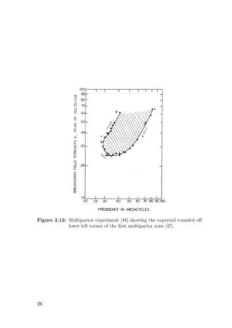
Page 20 and 21: to physically damage microwave comp
Page 22 and 23: odd positive integer (N = 1,3,5...)
Page 24 and 25: σ se [−] 2.5 2 1.5 1 0.5 W 1 W m
Page 26 and 27: Voltage [V] 10 4 10 3 10 2 10 0 N=1
Page 28 and 29: even though it may be sufficient fr
Page 30 and 31: where φL and φR are the left and
Page 32 and 33: (cf. Fig. 2.7). When taking the env
Page 34 and 35: 2.1.4 Methods of suppression Many o
Page 36 and 37: Noise (dBm) Power #1 (dBm) Match #1
Page 38 and 39: andom spread in emission velocities
Page 42 and 43: where kn is a factor determining th
Page 44 and 45: allows for another design margin, w
Page 46 and 47: Boundary function Method One of the
Page 48 and 49: carriers, because the NLSQ method r
Page 50 and 51: multipactor discharge. Using a Mont
Page 52 and 53: the assumption of a constant ratio
Page 54 and 55: Voltage (V) 10 3 10 2 10 1 10 −2
Page 56 and 57: 3.1.3 Main results The main result
Page 58 and 59: lytical model is obviously needed.
Page 60 and 61: where 〈vt 2 〉 represents the av
Page 62 and 63: these quantities in the range from
Page 64 and 65: analytical. Attempts were made to f
Page 66 and 67: only model, the inclusion of ionisa
Page 68 and 69: Normalised Voltage 1.1 1.05 1 0.95
Page 70 and 71: Voltage [V] 10 3 10 0 µ=0 µ=0.75
Page 73 and 74: Chapter 4 Multipactor in irises A c
Page 75 and 76: h l Figure 4.1: The geometry used i
Page 77 and 78: N e /N 0 [−] 3 2.5 2 1.5 1 Multip
Page 79 and 80: to compensate for electron losses i
Page 81: 4.4 Main results This analysis has
Page 84 and 85: support for the qualitative analyti
Page 86 and 87: where R(t) is the average position,
Page 88 and 89: where d stands for the gap width, V
Page 90 and 91:
there are different oscillatory vel
Page 92 and 93:
Phase [degrees] 60 50 40 30 20 10
Page 94 and 95:
G 100 90 80 70 60 50 40 30 20 10 0
Page 96 and 97:
possible for quite large Ro/Ri-valu
Page 98 and 99:
upper right region of the figures,
Page 100 and 101:
σse,max the zones become wider and
Page 102 and 103:
G 50 45 40 35 30 25 20 15 10 5 0.2
Page 104 and 105:
creasing ratio Ri/Ro was observed.
Page 107 and 108:
Chapter 6 Detection of multipactor
Page 109 and 110:
Amplitude of acceleration [Gm/s 2 ]
Page 111 and 112:
tipactor events that are short-live
Page 113 and 114:
software and the time evolution of
Page 115 and 116:
ditional test sample, a resonant ca
Page 117 and 118:
the FFT. It was concluded that ther
Page 119 and 120:
6.2.1 Single carrier When using the
Page 121 and 122:
Reference signal generator Phase co
Page 123 and 124:
Amplitude [A.U.] 2.5 2 1.5 1 0.5 De
Page 125 and 126:
Chapter 7 Conclusions and outlook T
Page 127 and 128:
tioned there were multipactor in no
Page 129 and 130:
References [1] W. Henneberg, R. Ort
Page 131 and 132:
[27] A. Ruiz et al, “Ti, V, and C
Page 133 and 134:
[51] D. Wolk, D. Schmitt, and T. Sc
Page 135 and 136:
[75] R. Udiljak, Multipactor in low
Page 137:
Included papers A-F 123
Page 141:
Paper B R. Udiljak, D. Anderson, M.
Page 145:
Paper D R. Udiljak, D. Anderson, M.
Page 149:
Paper F V. E. Semenov, N. Zharova,
show all

Multipactor in Low Pressure Gas and in ... - of Richard Udiljak

Create successful ePaper yourself

Delete template?

Save as template?