Bayesian Programming and Learning for Multi-Player Video Games ...

• AD1:n ∈ {no, low, med, high}: same for air defense.
• ID1:n ∈ {no detector, one detector, several}: invisible defense, equating to numbers of
detectors.
• T T ∈ [∅, building1, building2, building1 ∧ building2, techtrees, . . . ]: all the possible technological
trees for the given race. For instance {pylon, gate} and {pylon, gate, core} are
two different T ech T rees, see chapter 7.
• HP ∈ {ground, ground∧air, ground∧invis, ground∧air∧invis, ground∧drop, ground∧
air∧drop, ground∧invis∧drop, ground∧air∧invis∧drop}: how possible types of attacks,
directly mapped from T T information. This variable serves the purpose of extracting all
that we need to know from T T and thus reducing the complexity of a part of the model
from n mappings from T T to Hi to one mapping from T T to HP and n mapping from
HP to Hi. Without this variable, learning the co-occurrences of T T and Hi is sparse
in the dataset. In prediction, with this variable, we make use of what we can infer on
the opponent’s strategy Synnaeve and Bessière [2011b], Synnaeve and Bessière [2011], in
decision-making, we know our own possibilities (we know our tech tree as well as the units
we own).
We can consider a more complex version of this tactical model taking soft evidences into account
(variables on which we have a probability distribution), which is presented in appendix B.2.1.
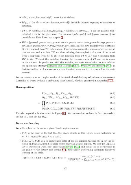
Decomposition
=
P(A1:n, E1:n, T1:n, T A1:n, B1:n, (6.1)
H1:n, GD1:n, AD1:n, ID1:n, HP, T T ) (6.2)
n�
[P(Ai)P(Ei, Ti, T Ai, Bi|Ai) (6.3)
i=1
P(ADi, GDi, IDi|Hi)P(Hi|HP )] P(HP |T T )P(T T ) (6.4)
This decomposition is also shown in Figure 6.4. We can see that we have in fact two models:
one for A1:n and one for H1:n.
Forms and learning
We will explain the forms for a given/fixed i region number:
• P(A) is the prior on the fact that the player attacks in this region, in our evaluation we
set it to nbattles/(nbattles + nnot battles).
• P(E, T, T A, B|A) is a co-occurrences table of the economical, tactical (both for the defender
and the attacker), belonging scores where an attacks happen. We just use Laplace’s
law of succession (“add one” smoothing) Jaynes [2003] and count the co-occurrences in
the games of the dataset (see section 6.4), thus almost performing maximum likelihood
learning of the table.
P(E = e, T = t, T A = ta, B = b|A = T rue) =
102
1 + nbattles(e, t, ta, b)
|E| |T | |T A| |B| + �
E,T,T A,B nbattles(E, T, T A, B)