Bayesian Programming and Learning for Multi-Player Video Games ...

M
Op t-1
M
Op t
V
T
0,1
BT O N
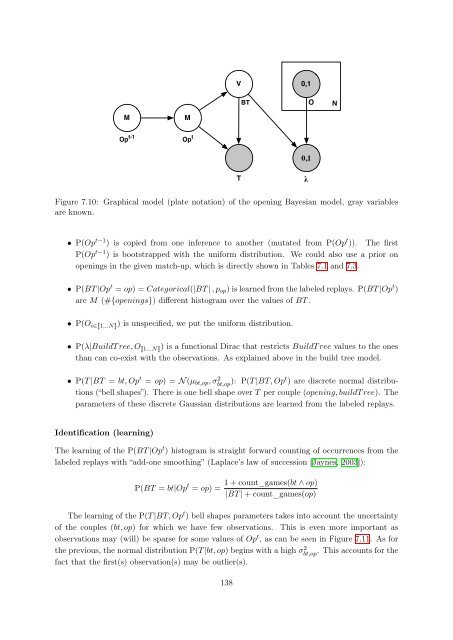
Figure 7.10: Graphical model (plate notation) of the opening Bayesian model, gray variables
are known.
• P(Op t−1 ) is copied from one inference to another (mutated from P(Op t )). The first
P(Op t−1 ) is bootstrapped with the uniform distribution. We could also use a prior on
openings in the given match-up, which is directly shown in Tables 7.1 and 7.3.
• P(BT |Op t = op) = Categorical(|BT | , pop) is learned from the labeled replays. P(BT |Op t )
are M (#{openings}) different histogram over the values of BT .
• P(O i∈�1...N�) is unspecified, we put the uniform distribution.
• P(λ|BuildT ree, O �1...N�) is a functional Dirac that restricts BuildT ree values to the ones
than can co-exist with the observations. As explained above in the build tree model.
• P(T |BT = bt, Op t = op) = N (µbt,op, σ 2 bt,op ): P(T |BT, Opt ) are discrete normal distributions
(“bell shapes”). There is one bell shape over T per couple (opening, buildT ree). The
parameters of these discrete Gaussian distributions are learned from the labeled replays.
Identification (learning)
The learning of the P(BT |Op t ) histogram is straight forward counting of occurrences from the
labeled replays with “add-one smoothing” (Laplace’s law of succession [Jaynes, 2003]):
P(BT = bt|Op t = op) =
0,1
1 + count_games(bt ∧ op)
|BT | + count_games(op)
The learning of the P(T |BT, Opt ) bell shapes parameters takes into account the uncertainty
of the couples (bt, op) for which we have few observations. This is even more important as
observations may (will) be sparse for some values of Opt , as can be seen in Figure 7.11. As for
the previous, the normal distribution P(T |bt, op) begins with a high σ2 bt,op . This accounts for the
fact that the first(s) observation(s) may be outlier(s).
138
λ