Bayesian Programming and Learning for Multi-Player Video Games ...

μ
σ
K'
K'
EC t
EU
Q
Army mixture
(GMM)
What we infer
V'
ETT
What we see What we want to know
EU
What we want
to do (tactics)
U
K'
K' K K
V
EC t
K
EC t+1 C c
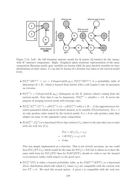
Figure 7.14: Left: the full Gaussian mixture model for Q armies (Q battles) for the enemy,
with K ′ mixtures components. Right: Graphical (plate notation) representation of the army
composition Bayesian model, gray variables are known while for gray hatched variables we have
distributions on their values. Ct can also be known (if a decision was taken at the tactical model
level).
• P(C t+1
c |EC t+1 = ec) = Categorical(K, pec), P(C t+1
c |EC t+1 ) is a probability table of
dimensions K × K ′ , which is learned from battles with a soft Laplace’s law of succession
on victories.
• P(C t+1
t ) = Categorical(K, ptac) (histogram on the K clusters values) coming from the
tactical model. Note that it can be degenerate: P(C t+1
t = shuttle) = 1.0. It serves the
purpose of merging tactical needs with strategic ones.
• P(C t+1
m |C t+1
t
, C t+1
c ) = αP(C t+1
t )+(1−α)P(Ct+1 c ) with α ∈ [0 . . . 1] the aggressiveness/ini-
tiative parameter which can be set fixed, learned, or be variable (P (α|situation)). If α = 1
we only produce units wanted by the tactical model, if α = 0 we only produce units that
adapts our army to the opponent’s army composition.
• P(λ|C t+1
f , C t+1
m ) is a functional Dirac that restricts Cm values to the ones that can co-exist
with our tech tree (Cf ).
C t
P(λ = 1|Cf , Cm = cm)
= 1 iff P(Cf = cm) �= 0
= 0 else
This was simply implemented as a function. This is not strictly necessary (as one could
have P(Cf |T T, Cm) which would do the same for P(Cf ) = 0.0) but it allows us to have the
same table form for P(Cf |T T ) than for P(EC|ET T ), should we wish to use the learned
co-occurrences tables (with respect to the good race).
• P(C t+1
f |T T ) is either a learned probability table, as for P (EC t+1 |ET T t ), or a functional
Dirac distribution which tells which Cf values (cf ) are compatible with the current tech
tree T T = tt. We used this second option. A given c is compatible with the tech tree
148
C f
K
C m
TT
0,1
λ
What we have