Bayesian Programming and Learning for Multi-Player Video Games ...

7.6 Openings
7.6.1 Bayesian model
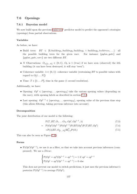
We now build upon the previous build tree* predictor model to predict the opponent’s strategies
(openings) from partial observations.
Variables
As before, we have:
• Build trees: BT ∈ [∅, building1, building2, building1 ∧ building2, techtrees, . . . ]: all
the possible building trees for the given race. For instance {pylon, gate} and
{pylon, gate, core} are two different BT .
• N Observations: O i∈�1...N� ∈ {0, 1}, Ok is 1 (true) if we have seen (observed) the kth
building (it can have been destroyed, it will stay “seen”).
• Coherence variable: λ ∈ {0, 1}: coherence variable (restraining BT to possible values with
regard to O �1 . . . N�)
• Time: T ∈ �1 . . . P �, time in the game (1 second resolution).
Additionally, we have:
• Opening: Op t ∈ [opening1 . . . openingM] take the various opening values (depending on
the race), with opening labels as described in section 7.3.2.
• Last opening: Op t−1 ∈ [opening1 . . . openingM], opening value of the previous time step
(this allows filtering, taking previous inference into account).
Decomposition
The joint distribution of our model is the following:
This can also be seen as Figure 7.10.
Forms
P(T, BT, O1 . . . ON, Op t , Op t−1 , λ) (7.3)
= P(Op t |Op t−1 )P(Op t−1 )P(BT |Op t )P(T |BT, Op t ) (7.4)
×P(λ|BT, O �1...N�)Π N i=1P(Oi) (7.5)
• P(Opt |Opt−1 ), we use it as a filter, so that we take into account previous inferences (compressed).
We use a Dirac:
⎧
⎨
⎩
P(Op t = op t |Op t−1 = op t−1 ) = 1 if op t = op t−1
P(Op t = op t |Op t−1 = op t−1 ) = 0 else
This does not prevent our model to switch predictions, it just uses the previous inference’s
posterior P(Op t−1 ) to average P(Op t ).
137