Bayesian Programming and Learning for Multi-Player Video Games ...

which derives the laws of probability: the “product-rule” (P(A, B) = P(A ∩ B) = P(A|B)P(B))
and the “sum-rule” (P(A+B) = P(A)+P(B)−P(A, B) or P(A∪B) = P(A)+P(B)−P(A∩B))
of probabilities.
Indeed, this was proved by Cox [1946], producing Cox’s theorem (also named Cox-Jayne’s
theorem):
Theorem. A system for reasoning which satisfies:
• divisibility and comparability, the plausibility of a statement is a real number,
• common sense, in presence of total information, reasoning is isomorphic to Boolean logic,
• consistency, two identical mental states should have the same degrees of plausibility,
is isomorphic to probability theory.
So, the degrees of belief, of any consistent induction mechanism, verify Kolmogorov’s axioms.
Finetti [1937] showed that if reasoning is made in a system which is not isomorphic to probability
theory, then it is always possible to find a Dutch book (a set of bets which guarantees a profit
regardless of the outcomes). In our quest for a consistent reasoning mechanism which
is able to deal with (extensional and intentional) uncertainty, we are thus bound to
probability theory.
3.2.2 A formalism for Bayesian models
Inspired by plausible reasoning, we present Bayesian programming, a formalism that can be used
to describe entirely any kind of Bayesian model. It subsumes Bayesian networks and Bayesian
maps, as it is equivalent to probabilistic factor graphs Diard et al. [2003]. There are mainly two
parts in a Bayesian program (BP)*, the description of how to compute the joint distribution,
and the question(s) that it will be asked.
The description consists in exhibiting the relevant variables {X 1 , . . . , X n } and explain their
dependencies by decomposing the joint distribution P(X 1 . . . X n |δ, π) with existing preliminary
(prior) knowledge π and data δ. The forms of each term of the product specify how to compute
their distributions: either parametric forms (laws or probability tables, with free parameters
that can be learned from data δ) or recursive questions to other Bayesian programs.
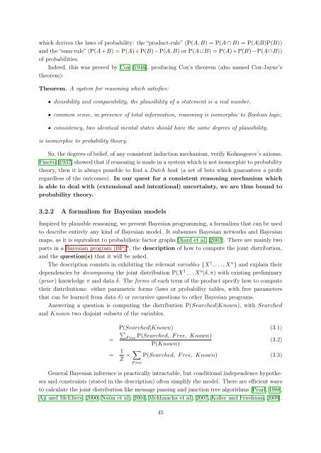
Answering a question is computing the distribution P(Searched|Known), with Searched
and Known two disjoint subsets of the variables.
=
P(Searched|Known) (3.1)
�
F ree
P(Searched, F ree, Known)
P(Known)
(3.2)
= 1 �
× P(Searched, F ree, Known) (3.3)
Z
F ree
General Bayesian inference is practically intractable, but conditional independence hypotheses
and constraints (stated in the description) often simplify the model. There are efficient ways
to calculate the joint distribution like message passing and junction tree algorithms [Pearl, 1988,
Aji and McEliece, 2000, Naïm et al., 2004, Mekhnacha et al., 2007, Koller and Friedman, 2009].
45