Bayesian Programming and Learning for Multi-Player Video Games ...

Recommendations

Info

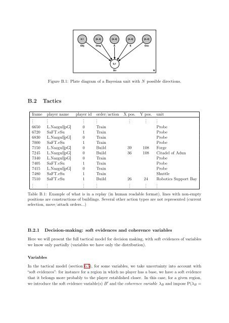
B.2 Tactics 0,1 Obj [0..3] Dmg [0..2] A 0,1 Dir Figure B.1: Plate diagram of a Bayesian unit with N possible directions. frame player name player id order/action X pos. Y pos. unit . . . . . . . 6650 L.Nazgul[pG] 0 Train Probe 6720 SaFT.eSu 1 Train Probe 6830 L.Nazgul[pG] 0 Train Probe 7000 SaFT.eSu 1 Train Probe 7150 L.Nazgul[pG] 0 Build 39 108 Forge 7245 L.Nazgul[pG] 0 Build 36 108 Citadel of Adun 7340 L.Nazgul[pG] 0 Train Probe 7405 SaFT.eSu 1 Train Probe 7415 L.Nazgul[pG] 0 Train Probe 7480 SaFT.eSu 1 Train Shuttle 7510 SaFT.eSu 1 Build 26 24 Robotics Support Bay . . . . Table B.1: Example of what is in a replay (in human readable format), lines with non-empty positions are constructions of buildings. Several other action types are not represented (current selection, move/attack orders...) B.2.1 Decision-making: soft evidences and coherence variables Here we will present the full tactical model for decision making, with soft evidences of variables we know only partially (variables we have only the distribution). Variables In the tactical model (section 6.5), for some variables, we take uncertainty into account with “soft evidences”: for instance for a region in which no player has a base, we have a soft evidence that it belongs more probably to the player established closer. In this case, for a given region, we introduce the soft evidence variable(s) B ′ and the coherence variable λB and impose P(λB = [0..2] . E [0..2] Occ . N .
1|B, B ′ ) = 1.0 iff B = B ′ , else P(λB = 1|B, B ′ ) = 0.0; while P(λB|B, B ′ )P(B ′ ) is a new factor in the joint distribution. This allows to sum over P(B ′ ) distribution (soft evidence). We do that for all the variables which will not be directly observed in decision-making. Decomposition The joint distribution of our model contains soft evidence variables for all input family variables (E, T, B, GD, AD, ID) as we cannot know for sure the economical values of the opponent’s regions under the fog of war* (E), nor can we know exactly the tactical value (T ) for them, nor the possession of the regions (B), nor the exact defensive scores (GD, AD, ID). Under this form, it deals with all possible uncertainty (from incomplete information) that may come up in a game. For the n considered regions, we have: Forms = P(A1:n, E1:n, T1:n, T A1:n, B1:n, B ′ 1:n, λB,1:n, T ′ 1:n, λT,1:n, (B.1) E ′ 1:n, λE,1:n, ID ′ 1:n, λID,1:n, GD ′ 1:n, λGD,1:n, AD ′ 1:n, λAD,1:n, (B.2) H1:n, GD1:n, AD1:n, ID1:n, HP, T T ) (B.3) n� [P(Ai)P(Ei, Ti, T Ai, Bi|Ai) (B.4) i=1 P(λB,i|B1:n, B ′ 1:n)P(B ′ 1:n)P(λT,i|T1:n, T ′ 1:n)P(T ′ 1:n) (B.5) P(λE,i|E1:n, E ′ 1:n)P(E ′ 1:n)P(λID,i|ID1:n, ID ′ 1:n)P(ID ′ 1:n) (B.6) P(λGD,i|GD1:n, GD ′ 1:n)P(GD ′ 1:n)P(λAD,i|AD1:n, AD ′ 1:n)P(AD ′ 1:n) (B.7) P(ADi, GDi, IDi|Hi)P(Hi|HP )] P(HP |T T )P(T T ) (B.8) The full plate diagram of this model is shown in Figure B.6. To the previous forms (section 6.5.1), we add for all variables which were doubles (X with X ′ ): ⎧ ⎨ Identification P(λX|X, X ′ ) = 1.0 iff X = X ′ ⎩P(λX|X, X ′ ) = 0.0 else The identification and learning does not change, c.f. section 6.5.1. Questions ∝ ∝ ∀i ∈ regions P(Ai|tai, λB,i = 1, λT,i = 1, λE,i = 1) � � � B i,B ′ i T i,T ′ i E i,E ′ i P(Ei, Ti, tai, Bi|Ai)P(Ai)P(B ′ i)P(T ′ i )P(E ′ i) ∀i ∈ regions P(Hi|tt, λID,i = 1, λGD,i = 1, λAD,i = 1) � � � � ID i,ID ′ i GD i,GD ′ i ADi,AD ′ i HP P(ADi, GDi, IDi|Hi)P(Hi|HP )P(HP |tt)P(ID ′ i)P(AD ′ i)P(GD ′ i) 199
Page 1:
THÈSE Pour obtenir le grade de DOC
Page 4 and 5:
Contents Contents 4 1 Introduction
Page 6 and 7:
5.4.1 Bayesian unit . . . . . . . .
Page 8 and 9:
Notations Symbols ← assignment of
Page 10 and 11:
Complexity, real-time constraints a
Page 12 and 13:
intuition of Bayesian modeling to r
Page 14 and 15:
e played by humans, by opposition t
Page 16 and 17:
As a first approach, programmers ca
Page 18 and 19:
3 2 1 1 Figure 2.1: A Tic-tac-toe b
Page 20 and 21:
Algorithm 2 Alpha-beta algorithm fu
Page 22 and 23:
ewards on all the runs through node
Page 24 and 25:
2.4.1 Monopoly In Monopoly, there i
Page 26 and 27:
2.4.3 Poker Poker 4 is a zero-sum (
Page 28 and 29:
2.5.2 State of the art FPS AI consi
Page 30 and 31:
2.6.2 State of the art Methods used
Page 32 and 33:
are no generic and efficient approa
Page 34 and 35:
Strategy Tactics Action Strategic d
Page 36 and 37:
2.8.4 Time constant(s) For novice t
Page 38 and 39:
effects. In RTS games, there is a l
Page 41 and 42:
Chapter 3 Bayesian modeling of mult
Page 43 and 44:
programmer-specified states, the (m
Page 45 and 46:
which derives the laws of probabili
Page 47 and 48:
Indeed, when evaluating two models
Page 49 and 50:
• energy/mana/stamina regenerator
Page 51 and 52:
• The probability that the ith un
Page 53 and 54:
3.3.4 Example This model has been a
Page 55 and 56:
and P(Ai = false|T = i) = 0.6. To m
Page 57 and 58:
Chapter 4 RTS AI: StarCraft: Broodw
Page 59 and 60:
eplay is shown in appendix in Table
Page 61 and 62:
Supply/Max supply Build Note (popul
Page 63 and 64:
Figure 4.3: Military moves from a S
Page 65 and 66:
Technology Strategy Army How? Econo
Page 67:
• Robotic player (bot): chapter 8
Page 70 and 71:
• Complexity: pspace-complete [Pa
Page 72 and 73:
educing the complexity (no communic
Page 74 and 75:
(grid-based) pathfinding was recent
Page 76 and 77:
U A E Figure 5.4: In both figures,
Page 78 and 79:
Fire Reload Figure 5.6: Fight FSM o
Page 80 and 81:
• Obj i∈�1...n� ∈ {T rue,
Page 82 and 83:
Identification Parameters and proba
Page 84 and 85:
⎧⎪ Bayesian program ⎨ ⎧⎪
Page 86 and 87:
36 units setup vs OAI. For Bayesian
Page 88 and 89:
we learned, by optimizing the effic
Page 90 and 91:
Probabilistic modality Finally, we
Page 92 and 93:
• Type: prediction is problem of
Page 94 and 95:
can possibly be in the future. In t
Page 96 and 97:
6.3.2 Evaluating regions Partial ob
Page 98 and 99:
Pylon Gate Core Range Gate Core Pyl
Page 100 and 101:
events (detected by a heuristic, se
Page 102 and 103:
• AD1:n ∈ {no, low, med, high}:
Page 104 and 105:
The model is highly modular, and so
Page 106 and 107:
attacked: P(ei�=r, ti�=r, tai
Page 108 and 109:
Figure 6.7: P(A) for varying values
Page 110 and 111:
Towards a baseline heuristic The me
Page 112 and 113:
Figure 6.9 displays the mean P(A, H
Page 114 and 115:
Finally, our approach is not exclus
Page 117 and 118:
Chapter 7 Strategy Strategy without
Page 119 and 120:
etween economy, technology and mili
Page 121 and 122:
power to the player (it allows for
Page 123 and 124:
7.4.2 Probabilistic labeling Instea
Page 125 and 126:
• Variables: - X i∈�1...n�
Page 127 and 128:
Figure 7.3: Protoss vs Terran distr
Page 129 and 130:
7.5 Build tree prediction The work
Page 131 and 132:
Questions The question that we will
Page 133 and 134:
Table 7.4 shows the full results, t
Page 135 and 136:
that this average “missed” (unp
Page 137 and 138:
7.6 Openings 7.6.1 Bayesian model W
Page 139 and 140:
Questions The question that we will
Page 141 and 142:
Figure 7.12: Evolution of P(Opening
Page 143 and 144:
Table 7.5: Prediction probabilities
Page 145 and 146:
7.6.3 Possible uses We recall that
Page 147 and 148: • U t+1 ∈ ([0, 1] . . . [0, 1])
Page 149 and 150: (tt) if it allows for building all
Page 151 and 152: 7.7.2 Results We did not evaluate d
Page 153 and 154: forces scores PvP PvT PvZ TvT TvZ Z
Page 155 and 156: shows a brutal transition from the
Page 157 and 158: Chapter 8 BroodwarBotQ Dealing with
Page 159 and 160: 8.1.2 Tactical goals The decision t
Page 161 and 162: • X t i∈�1...n� ∈ �r1 .
Page 163 and 164: 3 2 player 1 1 6 4 resources 8 play
Page 165 and 166: the construction plan as our Produc
Page 167 and 168: Figure 8.5: Crops of screenshots of
Page 169: anking). We consider that this rati
Page 172 and 173: This is an extension of the work on
Page 174 and 175: • differences in situations: as t
Page 176 and 177: 9.2.4 Inter-game Adaptation (Meta-g
Page 178 and 179: fog of war hiding of some of the fe
Page 180 and 181: RTS Real-Time Strategy games are (m
Page 182 and 183: Sander C. J. Bakkes, Pieter H. M. S
Page 184 and 185: Julien Diard, Pierre Bessière, and
Page 186 and 187: Damian Isla. Handling complexity in
Page 188 and 189: Kinshuk Mishra, Santiago Ontañón,
Page 190 and 191: Mark Riedl, Boyang Li, Hua Ai, and
Page 192 and 193: Adrien Treuille, Seth Cooper, and Z
Page 194 and 195: • 0 (not at all, or irrelevant)
Page 197: Appendix B StarCraft AI B.1 Micro-m
Page 201 and 202: Figure B.2: Top: StarCraft’s Lost
Page 203 and 204: 0,1 B' [0..5] T [0..2] E' 0,1 λ B
Page 205 and 206: C C A A C C A A 4 B B 4 3 4 B B 4 3
show all

Bayesian Programming and Learning for Multi-Player Video Games ...

You also want an ePaper? Increase the reach of your titles

Delete template?

Save as template?