Optimization and Computational Fluid Dynamics - Department of ...

250 Marco Manzan, Enrico Nobile, Stefano Pieri and Francesco Pinto
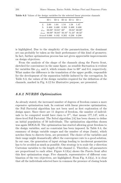
Table 8.3 Values of the design variables for the selected linear piecewise channels
ID i ID ii ID iii ID iv ID v
L 2.00 1.64 1.54 1.58 1.47
h 0.400 0.400 0.383 0.400 0.400
ϕin 60.00 ◦ 59.04 ◦ 60 ◦ 59.04 ◦ 60.00 ◦
ϕout 60.00 ◦ 56.04 ◦ 50.16 ◦ 51.24 ◦ 49.32 ◦
transl 0.066 0.102 0.202 0.236 0.298
is highlighted. Due to the simplicity of the parametrization, the dominant
set can probably be taken as the limit performance of this kind of geometry.
In fact, further optimization process has not given appreciable improvements
on design objectives.
From the analysis of the shape of the channels along the Pareto front,
sketched for convenience in the same figure, no sensible fluctuation is evident
for variables like ϕin and h, whichremaincloseto60 ◦ and 0.4, respectively.
What makes the difference is the translation of the upper profile, responsible
for the development of the separation bubble induced by the corrugation. In
Table 8.3, the values of the design variables required for the definition of the
channels, marked in Fig. 8.12 for illustrative purpose, are presented.
8.8.2 NURBS Optimization
As already stated, the increased number of degrees of freedom causes a more
expensive optimization task. In contrast with linear piecewise optimization,
the Full Factorial algorithm has not been used as first exploration of the
design space. Since there are 11 degrees of freedom, the number of individuals
to be computed would have risen to 3 11 , that means 177, 147, with a
three-level Full Factorial. The Sobol algorithm [14] has been chosen to define
an initial population of 50 individuals. The optimization algorithm chosen
was again MOGA-II. The optimization has started allowing great freedom to
the design variables, and no constraint has been imposed. In Table 8.4, the
summary of design variable ranges and the number of steps (basis), which
notches them to discrete form, are presented. The choice of the variables and
their range might dramatically affect the convergence rate to a good solution.
In our case, the generation of input strings leading to incoherent geometries
has to be avoided as much as possible. One strategy is to scale the x-direction
Cartesian variables to the length of the channel L. Therefore, all parameters
are proportional to each other. Figure 8.13(a) shows the Pareto front after
this first optimization stage. Five channels, representative of different combination
of the two objectives, are highlighted. From Fig. 8.13(a), it is clear
that all the individuals selected have in common the presence of closing bends