Introduzione ai modelli lineari - Analisi statistica ... - Docente.unicas.it

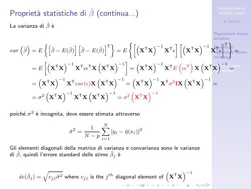
Proprietà statistiche di ˆβ (continua...)La varianza di ˆβ è( ) { [ ] [ ] } Tvar ˆβ = E ˆβ − E( ˆβ) ˆβ − E( ˆβ)Introduzione aimodelli lineariA. IodiceRegressione linearesemplice{ [( [ −1 ( ] }−1 TModello di= E X X) T X ɛ] T X X) T X regressione T ɛ = linearemultipla[ ( −1 ( ) ] −1 ( −1 (= E X X) T X T ɛɛ T X X T X = X X) T X T E ɛɛ T) (X(=X T X) −1X T var(ɛ)X= σ 2 ( X T X) −1X T X( ) −1 (X T X =(X X) ( −1 ) −1T = σ2X T XX T X) −1X T σ 2 IX(X T X) −1=Obiettivi −1dellaX X) Tregressione =poiché σ 2 è incognita, deve essere stimata attraversoˆσ 2 = 1N − pN∑[y i − ˆη(x i )] 2i=1Gli elementi diagonali della matrice di varianza e convarianza sono le varianzedi ˆβ, quindi l’errore standard delle stime ˆβ j èŝe( ˆβ√( ) −1j ) = c jj ˆσ 2 where c jj is the j th diagonal element of X T X