david queiroz de sant'ana avaliação acústica de edifícios religiosos ...

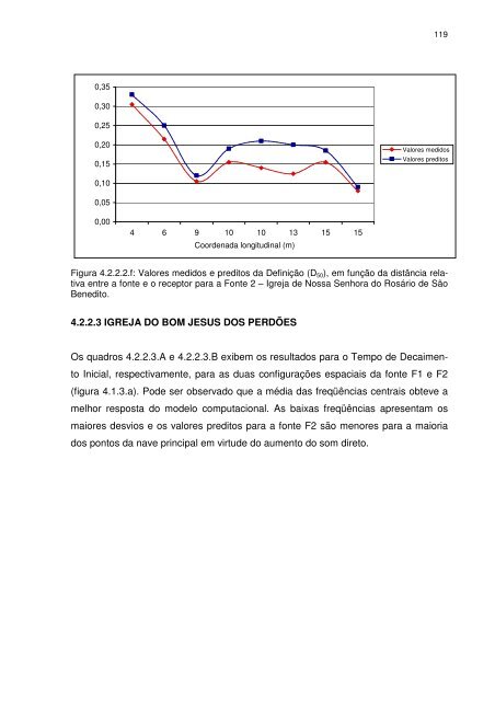
119
0,35
0,30
0,25
0,20
0,15
Valores medidos
Valores preditos
0,10
0,05
0,00
4 6 9 10 10 13 15 15
Coordenada longitudinal (m)
Figura 4.2.2.2.f: Valores medidos e preditos da Definição (D 50 ), em função da distância relativa
entre a fonte e o receptor para a Fonte 2 – Igreja de Nossa Senhora do Rosário de São
Benedito.
4.2.2.3 IGREJA DO BOM JESUS DOS PERDÕES
Os quadros 4.2.2.3.A e 4.2.2.3.B exibem os resultados para o Tempo de Decaimento
Inicial, respectivamente, para as duas configurações espaciais da fonte F1 e F2
(figura 4.1.3.a). Pode ser observado que a média das freqüências centrais obteve a
melhor resposta do modelo computacional. As baixas freqüências apresentam os
maiores desvios e os valores preditos para a fonte F2 são menores para a maioria
dos pontos da nave principal em virtude do aumento do som direto.