Statistik II für Statistiker, Mathematiker und Informatiker (SS ... - LMU

9. Schätzen 9.3 Konstruktion von Schätzfunktionen
9. Schätzen 9.3 Konstruktion von Schätzfunktionen
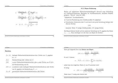
9.3.2 Bayes-Schätzung
⇒
∂ log L(µ,σ)
=
∂µ
∂ log L(µ,σ)
∂σ
=
⇒ ˆµ = ¯x, ˆσ =
n∑ x i − ˆµ
= 0
ˆσ 2
n∑
(− 1ˆσ + 2(x i − ˆµ) 2 )
= 0
2ˆσ 3
i=1
i=1
√
n∑
(x i − ¯x) 2
1
n
i=1
Basiert auf subjektivem Wahrscheinlichkeitsbegriff; dennoch enge Verbindung
zur Likelihood-Schätzung. Besonders für hochdimensionale, komplexe Modelle
geeignet; “Revival” etwa seit 1990.
“Subjektives” Grundverständnis:
• θ wird als Realisierung einer Zufallsvariablen Θ aufgefasst
• Unsicherheit/Unkenntnis über θ wird durch eine priori-Verteilung (stetige oder
diskrete Dichte)
f(θ)
bewertet. Meist: Θ stetige Zufallsvariable; f(θ) stetige Dichte.
Die Bayes-Inferenz beruht auf der posteriori-Verteilung von Θ, gegeben die Daten
x 1 , ...,x n . Dazu benötigen wir den Satz von Bayes für Dichten.
Statistik II für Statistiker, Mathematiker und Informatiker im SS 2007 148
Statistik II für Statistiker, Mathematiker und Informatiker im SS 2007 149
9. Schätzen 9.3 Konstruktion von Schätzfunktionen
Notation
f(x | θ) bedingte Wahrscheinlichkeitsfunktion bzw. Dichte von X, gegeben
Θ = θ
f(x) Randverteilung oder -dichte von X
f(θ) a priori Wahrscheinlichkeitsfunktion oder a priori Dichte von Θ (d.h.
die Randverteilung von Θ)
f(θ | x) a posteriori (oder bedingte) Wahrscheinlichkeitsfunktion oder Dichte
von Θ, gegeben die Beobachtung X = x
f(x,θ) gemeinsame Wahrscheinlichkeitsfunktion oder Dichte
9. Schätzen 9.3 Konstruktion von Schätzfunktionen
Dann gilt folgende Form des Satzes von Bayes:
Θ und X diskret:
⇒
f(θ | x) =
f(x, θ)
f(x)
=
P(X = x) = f(x) = ∑ j
f(x | θ)f(θ)
.
f(x)
f(x | θ j )f(θ j ) ,
wobei über die möglichen Werte θ j von Θ summiert wird.
Θ stetig:
⇒ f(θ | x) =
Dabei kann X stetig oder diskret sein.
f(x | θ)f(θ) f(x | θ)f(θ)
∫ = f(x | θ)f(θ)dθ f(x)
Statistik II für Statistiker, Mathematiker und Informatiker im SS 2007 150
Statistik II für Statistiker, Mathematiker und Informatiker im SS 2007 151