guidance, flight mechanics and trajectory optimization

More documents

Recommendations

Info

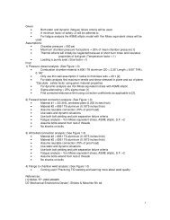
AGE a 0 1 2 3 4 5 6 7 8 9 10 Fl (a) DECISION K K K K K K K K K K K F3 (a) F2 (a) 19,000 17,000 15,000 13,000 11,000 9,000 9,000 9,000 9,000 9,000 9,000 DECISION K K K K K K R R R R R KEEP 27,000 24,000 21,000 18,000 15,000 14,000 13,000 12,000 11,000 10,000 I 9,000 REPLACE 17,000 17,000 17,000 17,000 17,000 17,000 17,000 17,000 17,000 17,000 17,000
The optimal policy can now be found by referring to the table. Note that the general solution is given; that is, the problem can begin with a machine of any age (not just 3 years old as in the original problem). This generality is the result of the fact that Dynamic Programming solves a class of problems rather than a specific problem. For a 15 stage process, the correct initial decision for the problem in which the machine is 3 years old is found in the grid 15 ( (Y ) <strong>and</strong> (Y = 3 (marked by a. For the next decision, Flrc (cr), the machine is 4 years old since it was kept for an additional year. The correct decision for this stage is again "keepl' as shown by the grid marked by 0 . The third decision is to Veplace" as shown by the grid labeled by 0. The fourth decision is shown by @ . The unit that was replaced in the third decision is one year old at the beginning of the fourth decision so the grid to use is F i2 ( Q! ) <strong>and</strong> a! = 1. This process continues as is shown by the remaining circ ed numbers. The final policy for the U-stage process that starts with a unit 3 years old is keep, keep, replace, keep, keep, keep, keep, replace, keep, keep, keep, replace, keep, keep, keep. The maximum profit for this problem is seen to be $91,000. Similarly, for 15 stages, the following table results: 46
Page 1 and 2: NASA OI 0 0 P; U 4 cd 4 z . . _ -.
Page 4: c FOREWORD This report was prepared
Page 7 and 8: SECTION PAGE 2.5 Dynamic Programmin
Page 10 and 11: 2.0 STATE OF THE ART 2.1 Developmen
Page 12 and 13: There are several ways to accomplis
Page 14 and 15: 2.2 Fundamental Concepts and Applic
Page 16 and 17: II. Although the previous problem w
Page 18 and 19: I,. Citg B. C optimum cost Path for
Page 20 and 21: The optimum path can be found by st
Page 22 and 23: The integral in Equation 2.2.1 can
Page 24 and 25: 2.2.2.1 Shortest Distance Between T
Page 26 and 27: The cost of the allowable transitio
Page 28 and 29: In a,completely analogous manner th
Page 30 and 31: 2.2.2.2 Variational Problem with Mo
Page 32 and 33: Ii _ 6 5 9 3 I 8 I I The cost integ
Page 34: 2.2.2.3 Simple Guidance Problem As
Page 37 and 38: This process continues in the same
Page 39 and 40: The algorithm for solving this prob
Page 41 and 42: The reader, no doubt, has a reasona
Page 43 and 44: are applied to Min (fl), the range
Page 45 and 46: Note that each diagonal corresponds
Page 47 and 48: The value of X can be found by empl
Page 49 and 50: The initial condition is: K.&P : P(
Page 51: it is seen that (for a two stage pr
Page 55 and 56: 2.3 COMPUTATIONAL CONSIDERATIONS So
Page 57 and 58: If classical techniques were to be
Page 59 and 60: 2.3.3.1 The Curse of Dimensionalitv
Page 61 and 62: Next, fl is evaluated for all allow
Page 63 and 64: % Xl + 5 = 2 (A2 = 2) 5+X2=3 (A2=3.
Page 65 and 66: that minimizes f. This interchange
Page 67 and 68: 2.3.3.2 Stability and Sensitivity I
Page 69 and 70: Let the lower limit of integration
Page 71 and 72: But (2.4.10) since the function on
Page 73 and 74: Now,. noting that the second MIN op
Page 75 and 76: where v 'is determined from and wit
Page 77 and 78: NOW, combining these two expression
Page 79 and 80: The situation is pictured to the ri
Page 81 and 82: Hence, the boundary condition OAI f
Page 83 and 84: The boundary condition to be satisf
Page 85 and 86: 2.4.7. Discussion of the Probltsi o
Page 87 and 88: characteristics associated with Eqs
Page 89 and 90: 2.4.8 The Problem of Bolza The prec
Page 91 and 92: The initial position, velocity and
Page 93 and 94: where I is the moment of inertia, F
Page 95 and 96: or, as . -... .-. . .._-_--- to ind
Page 97 and 98: Since R(t, x(t) ) is the minimum va
Page 99 and 100: 2.4.10 Ljnear Problem with Quadrati
Page 101 and 102: where S(t) is some n x n symmetric
Page 103 and 104:
The governing equations for the att
Page 105 and 106:
y 2.4.11 Dynamic Programming and th
Page 107 and 108:
M Since 3t does not depend on u exp
Page 109 and 110:
with The P vector for the system is
Page 111 and 112:
where With the control known as a f
Page 113 and 114:
with and with the boundary conditio
Page 115 and 116:
2.5 DYNAMIC PROGRAMMING AND THE OPT
Page 117 and 118:
2.5.2 Problem Statement Let the sys
Page 119 and 120:
Now, introducing the variables qs2,
Page 121 and 122:
Thus, the performance index takes t
Page 123 and 124:
#R where tr denotes the trace of th
Page 125 and 126:
The minimum value of the performanc
Page 127 and 128:
variance characterizing Ilt) can be
Page 129 and 130:
The solution takes the form with s
Page 131 and 132:
Since V is positive definite for f
Page 133 and 134:
where the first the second with exp
Page 135 and 136:
Taking the limit and using the expr
Page 137 and 138:
Since V is positive definite for t
Page 139 and 140:
2.5.3 The Treatment of Terminal Con
Page 141 and 142:
F while Equation (2.5.87B) requires
Page 143 and 144:
._ __. ..- . . - which will equal t
Page 145 and 146:
is determined. Let p(z,t') be given
Page 147 and 148:
of the p and $ equations (i.e., Eqs
Page 149 and 150:
(2.5.I.21) Thus, the control is to
Page 151 and 152:
Note, as in.Section (2.5.2.3), the
Page 153 and 154:
.6 t -(h.(S~tj~fitr~f-‘~~~~n~) =
Page 155 and 156:
3.0 RECOMMENDED PROCEDURES - ._ .-_
Page 157 and 158:
4 Section 2.5 (2.5.1) (2.5.2) (2.5.
show all

guidance, flight mechanics and trajectory optimization

You also want an ePaper? Increase the reach of your titles

Delete template?

Save as template?