Casestudie Breakdown prediction Contell PILOT - Transumo

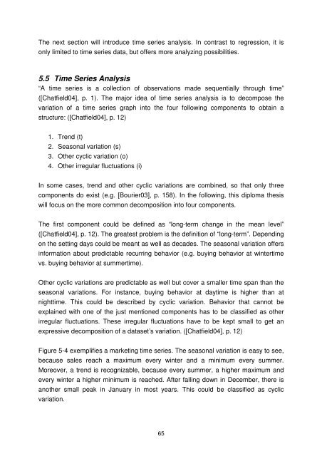
The next section will introduce time series analysis. In contrast to regression, it is
only limited to time series data, but offers more analyzing possibilities.
5.5 Time Series Analysis
“A time series is a collection of observations made sequentially through time”
([Chatfield04], p. 1). The major idea of time series analysis is to decompose the
variation of a time series graph into the four following components to obtain a
structure: ([Chatfield04], p. 12)
1. Trend (t)
2. Seasonal variation (s)
3. Other cyclic variation (o)
4. Other irregular fluctuations (i)
In some cases, trend and other cyclic variations are combined, so that only three
components do exist (e.g. [Bourier03], p. 158). In the following, this diploma thesis
will focus on the more common decomposition into four components.
The first component could be defined as “long-term change in the mean level”
([Chatfield04], p. 12). The greatest problem is the definition of “long-term”. Depending
on the setting days could be meant as well as decades. The seasonal variation offers
information about predictable recurring behavior (e.g. buying behavior at wintertime
vs. buying behavior at summertime).
Other cyclic variations are predictable as well but cover a smaller time span than the
seasonal variations. For instance, buying behavior at daytime is higher than at
nighttime. This could be described by cyclic variation. Behavior that cannot be
explained with one of the just mentioned components has to be classified as other
irregular fluctuations. These irregular fluctuations have to be kept small to get an
expressive decomposition of a dataset’s variation. ([Chatfield04], p. 12)
Figure 5-4 exemplifies a marketing time series. The seasonal variation is easy to see,
because sales reach a maximum every winter and a minimum every summer.
Moreover, a trend is recognizable, because every summer, a higher maximum and
every winter a higher minimum is reached. After falling down in December, there is
another small peak in January in most years. This could be classified as cyclic
variation.
65