T 7.2.1.3 Amplitude Modulation
T 7.2.1.3 Amplitude Modulation
T 7.2.1.3 Amplitude Modulation

You also want an ePaper? Increase the reach of your titles
YUMPU automatically turns print PDFs into web optimized ePapers that Google loves.
TPS <strong>7.2.1.3</strong><br />
Measuring instruments<br />
Fig. 2.1-4:The time law of electrical telecommunications engineering<br />
(A): Input signals: pulses with equal amplitude A and period T<br />
(B): Lowpasses with critical frequencies f c1<br />
and f c2<br />
; f c1<br />
< f c2<br />
(C): Output signals: pulse of varying period and amplitude<br />
If, for example, a spectrum analysis has to be performed<br />
over a wide frequency domain, and, in<br />
addition, a very short sawtooth period is selected,<br />
then the result of this is a very large change in frequency<br />
per unit time. The mixer output signal<br />
passes through the mid-frequencies of the BPF<br />
with corresponding speed. According to the time<br />
law the selected bandwidth of the BPF now has to<br />
be “sufficiently” large if the BPF is to attain the<br />
input amplitude. However, at greater bandwidth<br />
of the bandpass filter the analyzer's spectral resolution<br />
capacity drops. For that reason, work with<br />
the spectrum analyzer always involves the compromise<br />
between spectral RESOLUTION and<br />
fault-free reproduction of the amplitude. For the<br />
relationship between the SCAN TIME T, bandwidth<br />
b and frequency window SPAN the following<br />
approximately applies:<br />
b = 20 ( f − f )<br />
T<br />
max min (2.1)<br />
Where:<br />
f max : maximum frequency<br />
f min : minimum frequency<br />
b : bandwidth of the filter<br />
T : sawtooth period SCAN TIME.<br />
The difference f max – f min is called frequency<br />
window = SPAN.<br />
15