T 7.2.1.3 Amplitude Modulation

TPS 7.2.1.3
Double Sideband AM
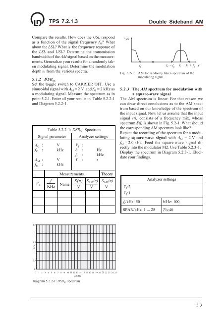
Compare the results. How does the USL respond
as a function of the signal frequency f M ? What
about the LSL? What is the frequency response of
the LSL and USL? Determine the transmission
bandwidth of the AM signal based on the measurements.
Generalize your results for a randomly taken
modulating signal. Determine the modulation
depth m from the various spectra.
5.2.2 DSB SC
Set the toggle switch to CARRIER OFF. Use a
sinusoidal signal with A M = 2 V and f M = 2 kHz as
a modulating signal. Measure the spectrum as in
point 5.2.1. Enter all your results in Table 5.2.2-1
and Diagram 5.2.2-1.
Table 5.2.2-1: DSB SC Spectrum
Signal parameter
Analyzer settings
A C : V V 1 :
f C : kHz b : Hz
f r : kHz
A M : V T : s
f M : kHz
s AM
f g f C – f g f C f C + f g
Fig. 5.2-1:
AM for randomly taken spectrum of the
modulating signal.
5.2.3 The AM spectrum for modulation with
a square-wave signal
The AM spectrum is linear. For that reason we
can draw direct conclusions as to the AM spectrum
based on our knowledge of the spectrum of
the input signal. Now let us assume that the input
signal s(t) consists of a frequency mix, whose
spectrum S(f) is shown in Fig. 5.2-1. What should
the corresponding AM spectrum look like?
Repeat the recording of the spectrum for a modulating
square-wave signal with A M = 2 V and
f M = 2.0 kHz. Feed the square-wave signal directly
into the modulator M2. Use Table 5.2.3-1.
Display the spectrum in Diagram 5.2.3-1. Elucidate
your findings.
f
V 2
f
KHz
Measurements
S( n)
Name
V
S AM (n)
V
Theory
S AM (n)
V
V 1 :2
V 2 :1
Analyzer settings
f r /kHz: 50 b/Hz: 100
SPAN/kHz: 1 ... 25
T/s:40
Diagram 5.2.2-1: DSB SC
spectrum
33