T 7.2.1.3 Amplitude Modulation

TPS 7.2.1.3
Review
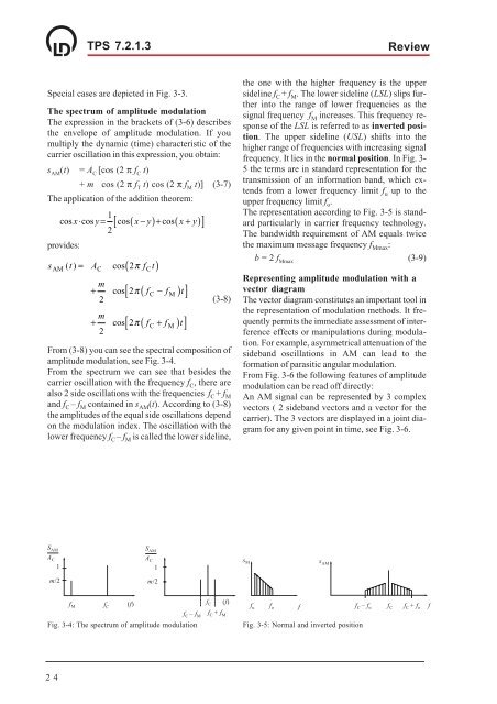
Special cases are depicted in Fig. 3-3.
The spectrum of amplitude modulation
The expression in the brackets of (3-6) describes
the envelope of amplitude modulation. If you
multiply the dynamic (time) characteristic of the
carrier oscillation in this expression, you obtain:
s AM
(t) = A C
[cos (2 π f C
t)
+ m cos (2 π f T
t) cos (2 π f M
t)] (3-7)
The application of the addition theorem:
1
cos x⋅ cos y= cos( x−y)+ cos x+
y
2
provides:
s ( t) A cos 2π
f t
AM C C
[ ( )]
= ( )
m
+ cos 2π
( fC
− fM
) t
2
[ ]
m
+ cos 2π
( fC
+ fM
) t
2
[ ]
(3-8)
From (3-8) you can see the spectral composition of
amplitude modulation, see Fig. 3-4.
From the spectrum we can see that besides the
carrier oscillation with the frequency f C , there are
also 2 side oscillations with the frequencies f C + f M
and f C – f M contained in s AM (t). According to (3-8)
the amplitudes of the equal side oscillations depend
on the modulation index. The oscillation with the
lower frequency f C – f M is called the lower sideline,
the one with the higher frequency is the upper
sideline f C + f M . The lower sideline (LSL) slips further
into the range of lower frequencies as the
signal frequency f M increases. This frequency response
of the LSL is referred to as inverted position.
The upper sideline (USL) shifts into the
higher range of frequencies with increasing signal
frequency. It lies in the normal position. In Fig. 3-
5 the terms are in standard representation for the
transmission of an information band, which extends
from a lower frequency limit f u up to the
upper frequency limit f o .
The representation according to Fig. 3-5 is standard
particularly in carrier frequency technology.
The bandwidth requirement of AM equals twice
the maximum message frequency f Mmax :
b = 2 f Mmax
(3-9)
Representing amplitude modulation with a
vector diagram
The vector diagram constitutes an important tool in
the representation of modulation methods. It frequently
permits the immediate assessment of interference
effects or manipulations during modulation.
For example, asymmetrical attenuation of the
sideband oscillations in AM can lead to the
formation of parasitic angular modulation.
From Fig. 3-6 the following features of amplitude
modulation can be read off directly:
An AM signal can be represented by 3 complex
vectors ( 2 sideband vectors and a vector for the
carrier). The 3 vectors are displayed in a joint diagram
for any given point in time, see Fig. 3-6.
S AM
S AM
A C
m/2
A C
m/2
f M f C
(f)
f C – f M
Fig. 3-4: The spectrum of amplitude modulation
s M
f u f o
s AM
f C – f o f C f C + f o
1
1
f C
f C + f M
(f)
f
Fig. 3-5: Normal and inverted position
f
24