Magnetic Fields and Magnetic Diagnostics for Tokamak Plasmas
Magnetic Fields and Magnetic Diagnostics for Tokamak Plasmas
Magnetic Fields and Magnetic Diagnostics for Tokamak Plasmas

Create successful ePaper yourself
Turn your PDF publications into a flip-book with our unique Google optimized e-Paper software.
<strong>Magnetic</strong> fields <strong>and</strong> tokamak plasmas<br />
Alan Wootton<br />
15. FULL EQUILIBRIUM RECONSTRUCTION<br />
The problem under discussion is how to reconstruct as much as is possible about the equilibrium<br />
from external measurements. In particular, if we knew everything about the fields outside the<br />
plasma, what could we uniquely determine Could we separate β I <strong>and</strong> l i (In principle yes <strong>for</strong><br />
toroidal systems). Could we go further <strong>and</strong> actually uniquely determine the plasma current<br />
distribution of a toroidal plasma (I don't know)<br />
If we want to allow measurements of dp(ψ)/dψ <strong>and</strong> FdF(ψ)/dψ we must have redundancy beyond<br />
that required to solve the equilibrium equation with a known current density profile. We see<br />
immediately a problem in straight geometry, because with straight circular cross sections the<br />
magnetic measurements must be consistent with a solution that has concentric circular surfaces.<br />
In this case the measurements are consistent with any profile function which gives the correct<br />
total plasma current, so there is an infinite degeneracy.<br />
In practice the mathematical subtleties of what can <strong>and</strong> cannot in principle be determined are not<br />
discussed. Instead the usual technique <strong>for</strong> equilibrium reconstruction is to choose a<br />
parameterization <strong>for</strong> j φ , with a restricted number of free parameters. These free parameters are<br />
chosen to minimize the chi squared error or cost function between some measured <strong>and</strong> computed<br />
parameter, <strong>for</strong> example the poloidal field component on some contour. Obviously we need some<br />
boundary conditions, as discussed in section 8. In<strong>for</strong>mation available might consist of the flux ψ<br />
on a contour, the fields B n <strong>and</strong> B τ on a contour, <strong>and</strong> currents in conductors, the total current, <strong>and</strong><br />
if lucky the diamagnetism. Typical parameterizations are<br />
⎡<br />
j φ<br />
= aβ R + ( 1− β) R ⎤<br />
0<br />
⎣<br />
⎢ R 0<br />
R ⎦<br />
⎥ g δψ<br />
( ) 15.1<br />
j φ<br />
= ( α 1<br />
δψ + α 2<br />
δψ 2 +α 3<br />
δψ 3<br />
)R + ( b 1<br />
δψ)R −1 15.2<br />
with δψ = (ψ-ψ boundary )(ψ mag axis -ψ boundary ). In each case the term proportional to R represent<br />
the part of j φ proportional to dp/dψ, <strong>and</strong> the part of j φ proportional to R -1 is proportional to<br />
FdF/dψ. R o is some characteristic radius. The assumed function g might be of the <strong>for</strong>m g(δψ,γ)<br />
= exp(-γ 2 (1-δψ) 2 , dψ γ or δψ + γδψ 2 . If in equation 15.1 the function g(δψ) is 1, then the<br />
description of j φ is called quasi uni<strong>for</strong>m: <strong>for</strong> a circular outer boundary there is an exact analytic<br />
solution of the equilibrium equation.<br />
113