Magnetic Fields and Magnetic Diagnostics for Tokamak Plasmas

Magnetic fields and tokamak plasmas
Alan Wootton
θ * =
φ = θ − a ⎛
β I
+ l i
q MHD
R ⎝
g
2 + 1 ⎞
⎠ sin( θ)
17.24
i.e. the perturbing fields must have the form (for r mn ≈ a)
⎛
b θ
= b mn
⎝
r mn
r
m +1
⎞
⎠
cos( mθ * + nφ − ω mn
t) 17.25
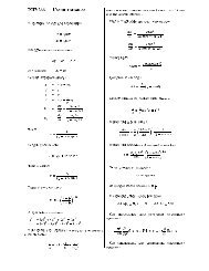
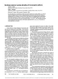
Figure 17.3 illustrates the field line trajectories in (φ,θ) space. Here we have assumed that
α
⎛
q MHD
( r) = q 0
+ q a
− q
⎞
0
, with q
⎝ ⎠ 0 the value at r = 0, q a the value at r = a (the plasma edge).
( ) r a
⎛
This allows us to express r = a⎜
q (r) − q MHD 0⎞
⎟
⎝ q a
− q 0
⎠
1
α
. In the figure we show examples for a = 0.25 m,
R g = 1 m, q 0 = 0.9, q a = 3.2, β I = 0.5, l i = 0.9. The solid lines are for q MHD = 3.2 (the plasma
edge), and the broken lines for q MHD = 2. The shear in the q profile is apparent.
φ
θ
Analysis techniques
outside
inside
Figure 17.3. The trajectory of field lines in φ, θ space for q = 2
(broken lines) and q = 3.2 (solid lines).
With a set of Mirnov coils spanning a poloidal cross section of a low beta, circular cross section
tokamak, we can take a Fourier transform in θ to obtain the amplitude of each component
cos(mθ+nφ-ω mn t). If we have a rectangular vessel, then we have shown that the relevant
expression is cos(mθ+θ+nφ-ω mn t). This has been done both computationally, and using analog
multiplexing. We should allow for the toroidal corrections discussed above when performing
this Fourier analysis; so that θ is replaced by θ*. Figure 17.4 shows the placement of the coils
124