Magnetic Fields and Magnetic Diagnostics for Tokamak Plasmas
Magnetic Fields and Magnetic Diagnostics for Tokamak Plasmas
Magnetic Fields and Magnetic Diagnostics for Tokamak Plasmas

Create successful ePaper yourself
Turn your PDF publications into a flip-book with our unique Google optimized e-Paper software.
<strong>Magnetic</strong> fields <strong>and</strong> tokamak plasmas<br />
Alan Wootton<br />
G 0<br />
( R, R' ) = µ 0<br />
kπ<br />
⎡ ⎛<br />
RR' E( k2)− ⎜ 1 − k2 ⎞<br />
⎣<br />
⎢ ⎝ 2 ⎠ K k2<br />
( )<br />
⎤<br />
⎦<br />
⎥<br />
8.16<br />
where<br />
k 2 =<br />
4RR'<br />
( R + R' ) 2 + ( z − z' ) 2<br />
( )<br />
8.17<br />
Ideal MHD<br />
Here we want to note only one important equation, which is a generalization of the “virial”<br />
equation. We use Equations 6.1, 1.1 <strong>and</strong> 1.2. Allow the total equilibrium field to be split up into<br />
two parts,<br />
B = B 1<br />
+ B 2<br />
8.18<br />
with ∇xB 2 = 0. We can choose the partitioning of B in a number of ways. Multiplying jxB =∇p<br />
by an arbitrary vector Q, we can obtain<br />
∫<br />
V<br />
⎡ ⎛<br />
⎜<br />
⎣<br />
⎢ ⎝<br />
p + B 2<br />
1<br />
⎞<br />
⎟ ∇• Q − B 1<br />
• ∇Q • B 1<br />
2µ 0<br />
⎠<br />
µ 0<br />
⎤<br />
dV<br />
⎦<br />
⎥<br />
⎡ ⎛<br />
= p + B 2<br />
⎜ 1<br />
⎞<br />
⎟<br />
(<br />
( Q • n) − B 1<br />
• Q)• ( B 1<br />
• n)<br />
⎤<br />
∫<br />
dS<br />
⎣<br />
⎢ ⎝ 2µ 0<br />
⎠<br />
µ 0 ⎦<br />
⎥ n<br />
−<br />
∫<br />
Q • ( j × B 2 )dV<br />
V<br />
S n<br />
8.19<br />
with n the normal to the surface S n . We have made use of the vector identity<br />
⎡<br />
Q[ ∇ × B • B]= ∇ • ( Q • B)B − B2<br />
⎣<br />
⎢ 2 Q ⎤<br />
⎦<br />
⎥ + B2<br />
2 ∇ • Q − B( B • ∇)Q<br />
We shall use equation 8.19 later to derive important integral relationships.<br />
Boundary conditions<br />
Last in this section we turn to boundary conditions. Suppose we have our three regions, as in<br />
Figure 8.2. Region 1 (S φplasma ) contains all the plasma current. Region 2 (S φvacuum ) contains no<br />
source, but contains a contour l on which we make measurements. Region 3 (S φcoils ) is outside<br />
region 2, extends to infinity, <strong>and</strong> contains all external currents. To find the plasma boundary we<br />
have to know ψ(R,z) in region 2 between the contour on which parameters are measured, <strong>and</strong> the<br />
plasma boundary itself. In principle we can do this knowing either<br />
82