Magnetic Fields and Magnetic Diagnostics for Tokamak Plasmas

Magnetic fields and tokamak plasmas
Alan Wootton
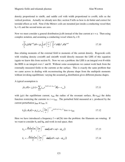
density proportional to sin(θ), and saddle coil with width proportional to cos(θ), tells us the
vertical position. Actually we already new this; section 9 tells us how to do better and correct for
toroidal effects as well. Note if the Mirnov coils are mounted just inside a conducting vessel then
b r = 0, and the second terms are zero.
Now we must consider a general distribution j(r,θ) instead of the line current at r = a. Then using
complex notation, and assuming a conducting vessel where b r = 0:
2π
r ∫ b θ
( θ ) e imθ ⎛
dθ = µ 0 ∫ dr'
⎝
0
r
0
r'
r
⎞
⎠
m 2π
∫ r' dθj( r' ,θ ) e imθ 17.10
0
thus relating moments of the external field to moments of the current density. Rogowski coils
with winding density cos(mθ) and sin(mθ) would directly measure the LHS of this equation
(again we knew this from section 9). Now we see a problem: the LHS is an integral over θ while
the RHS is an integral over r’ and θ. Without some assumptions we cannot work back from the
externally measured fields to the currents at the surface. This is exactly the same problem that
we came across in dealing with reconstructing the plasma shape from the multipole moments
without invoking equilibrium: varying the assumed j φ distribution gives different plasma shapes.
A typical assumption is
∑
j( r,θ)= j 0
( r) + j mn
e
m ,n
( )
δ r − rmn
i mθ +nφ −ω mnt
( ) 17.11
with j 0 (r) the equilibrium current, r mn the radius of the resonant surface, δ(r-r mn ) the delta
function restricting the currents to r = r mn . The perturbed field measured at r, produced by the
current perturbation j mn at r mn , is
b θ
m +1
⎛ r
( r,θ,φ) = µ 0
j mn
r mn ⎞
mn
⎝ r ⎠
e i( mθ +nφ −ω mn t)
for r > r mn 17.12
Here we have introduced a frequency f = ω/(2π) into the problem: the filaments are rotating. If
we want to consider b r and b θ , and work in real space, then
b θ
= µ 0
j mn
r mn
2
b r
= − µ 0
j mn
r mn
2
⎛ r mn
⎝ r
⎛ r mn
⎝ r
m +1
⎞
⎠
cos( mθ + nφ − ω mn
t) 17.13
m +1
⎞
⎠
sin( mθ + nφ − ω mn
t) 17.14
121