Magnetic Fields and Magnetic Diagnostics for Tokamak Plasmas

Magnetic fields and tokamak plasmas
Alan Wootton
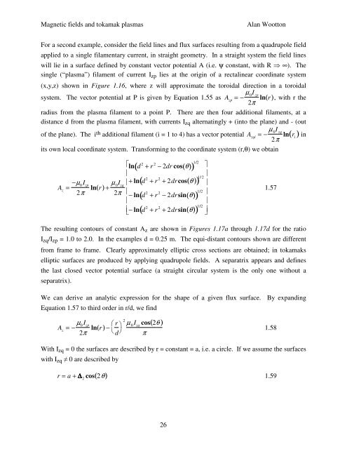
For a second example, consider the field lines and flux surfaces resulting from a quadrupole field
applied to a single filamentary current, in straight geometry. In a straight system the field lines
will lie in a surface defined by constant vector potential A (i.e. ψ constant, with R ⇒ ∞). The
single (“plasma”) filament of current I zp lies at the origin of a rectalinear coordinate system
(x,y,z) shown in Figure 1.16, where z will approximate the toroidal direction in a toroidal
system. The vector potential at P is given by Equation 1.55 as A zp
= − µ 0I zp
2π ln ( r ), with r the
radius from the plasma filament to a point P. There are then four additional filaments, at a
distance d from the plasma filament, with currents I zq alternatingly + (into the plane) and - (out
of the plane). The i th additional filament (i = 1 to 4) has a vector potential A zqi
= − µ 0I zq
2π ln ( r i
) in
its own local coordinate system. Transforming to the coordinate system (r,θ) we obtain
A z
= −µ 0 I zp
2π
ln( r)
+ µ I 0 zq
2π
( ) 1/2
⎡ ln d 2 + r 2 − 2dr cos( θ)
⎢
⎢ + ln d 2 + r 2 + 2drcos( θ )
⎢
− ln d 2 + r 2 − 2drsin( θ)
⎢
⎣
⎢ − ln d 2 + r 2 + 2drsin( θ)
( ) 1/ 2
( ) 1/2
( ) 1/2
⎤
⎥
⎥
⎥
⎥
⎦
⎥
1.57
The resulting contours of constant A z are shown in Figures 1.17a through 1.17d for the ratio
I zq /I zp = 1.0 to 2.0. In the examples d = 0.25 m. The equi-distant contours shown are different
from frame to frame. Clearly approximately elliptic cross sections are obtained; in tokamaks
elliptic surfaces are produced by applying quadrupole fields. A separatrix appears and defines
the last closed vector potential surface (a straight circular system is the only one without a
separatrix).
We can derive an analytic expression for the shape of a given flux surface. By expanding
Equation 1.57 to third order in r/d, we find
A z
= − µ 0
I zp
2π ln( r)
− ⎛ r ⎝ d
⎞
⎠
2
µ 0
I zq
cos( 2θ )
π
1.58
With I zq = 0 the surfaces are described by r = constant = a, i.e. a circle. If we assume the surfaces
with I zq ≠ 0 are described by
r = a + ∆ 2
cos( 2θ) 1.59
26