Quantum Field Theory I

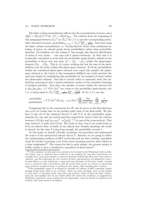
3.1. NAIVE APPROACH 95
1
2E jV
Thefinitevolumenormalizationaffectsalsothenormalizationofstates, since
〈⃗p|⃗p ′ 〉 = 2E ⃗p (2π) 3 δ 3 (⃗p−⃗p ′ ) → 2E ⃗p Vδ ⃗P P ⃗′. The relation from the beginning of
this paragraphbetween |S fi | 2 (or |T fi | 2 for f ≠ i) and the corresponding probability
thereforebecomes: probability for f≠i = |T fi | 2 ∏ n
j=1
. Note that using
the finite volume normalization, i.e. having discrete rather than continuous labeling
of states, we should speak about probabilities rather than probability
densities. Nevertheless, for the volume V big enough, this discrete distribution
of states is very dense — one may call it quasi-continuous. In that case it is
technically convenient to work with the probability quasi-density, defined as the
probability of decay into any state |f〉 = |⃗p 1 ,...,⃗p m 〉 within the phase-space
element d 3 p 1 ...d 3 p m . This is, of course, nothing else but the sum of the probabilities
over all states within this phase-space element. If all the probabilities
within the considered phase-space element were equal (the smaller the phasespace
element is, the better is this assumption fulfilled) one could calculate the
said sum simply by multiplying this probability by the number of states within
the phase-space element. And this is exactly what is commonly used (the underlying
reasoning is just a quasi-continuous version of the standard reasoning
of integral calculus). And since the number of states within the interval d 3 p
is ∆n x ∆n y ∆n z = V d 3 p/(2π) 3 one comes to the probability quasi-density (for
f ≠ i) being equal to |T fi | 2 ∏ n
j=1
1
2E jV
∏ m
k=1
probability
quasidensity = VT ∏
m
(2π)4 δVT(p 4 f −p i )|M fi | 2
V d 3 p
(2π) 3 . So for f ≠ i one has
j=1
d 3 p
(2π) 3 2E j
n ∏
j=m+1
1
2E j V .
Comparing this to the expressions for dΓ and dσ given in the Introductions
(see p.12) we realize that we are getting really close to the final result. We just
have to get rid of the awkward factors T and T/V in the probability quasidensities
for one and two initial particles respectively (and to find the relation
between 1/E A E B and [(p A .p B ) 2 −m 2 A m2 B ]−1/2 in caseofthe crosssection). This
step, however, is quite non-trivial. The point is that even if our result looks as
if we are almost done, actually we are almost lost. Frankly speaking, the result
is absurd: for the time T being long enough, the probability exceeds 1.
At this point we should critically reexamine our procedure and understand
the source of the unexpected obscure factor T. Instead, we are going to follow
the embarrassing tradition of QFT textbooks and use this evidently unreliable
result for further reasoning, even if the word reasoning used for what follows is
a clear euphemism 26 . The reason for this is quite simple: the present author is
boldly unable to give a satisfactory exposition of these issues 27 .
26 A fair comment on rates and cross sections is to be found in the Weinberg’s book (p.134):
The proper way to approach these problems is by studying the way that experiments are
actually done, using wave packets to represent particles localized far from each other before a
collision, and then following the time history of these superpositions of multiparticle states.
In what follows we will instead give a quick and easy derivation of the main results, actually
more a mnemonic than a derivation, with the excuse that (as far as I know) no interesting
open questions in physics hinge on getting the fine points right regarding these matters.
27 This incapability seems to be shared by virtually all authors of QFT textbooks (which
perhaps brings some relief to any of them). There are many attempts, more or less related
to each other, to introduce decay rates and cross sections. Some of them use finite volume,
some use wave-packets (but do not closely follow the whole time evolution, as suggested by
Weinberg’s quotation), some combine the two approaches. And one feature is common to all
of them: they leave much to be desired.