Quantum Field Theory I

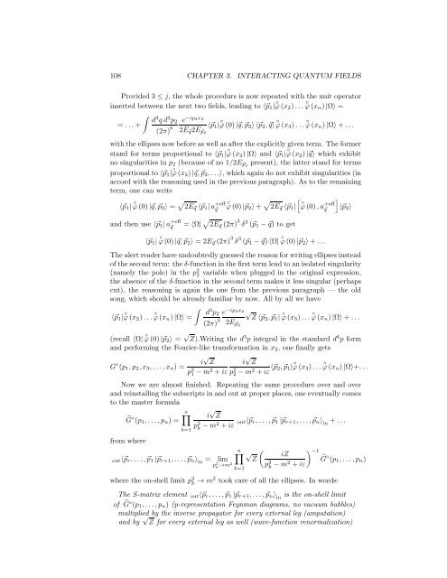
108 CHAPTER 3. INTERACTING QUANTUM FIELDS
Provided 3 ≤ j, the whole procedure is now repeated with the unit operator
inserted between the next two fields, leading to 〈⃗p 1 | ϕ(x ◦ 2 )... ϕ(x ◦ n )|Ω〉 =
∫ d 3 qd 3 p 2 e −ip2x2
= ...+
(2π) 6 〈⃗p 1 | ϕ(0)|⃗q,⃗p ◦ 2 〉〈⃗p 2 ,⃗q| ϕ(x ◦ 3 )... ϕ(x ◦ n )|Ω〉+...
2E ⃗q 2E ⃗p2
withthe ellipsesnowbeforeaswellasaftertheexplicitlygiventerm. Theformer
stand for terms proportional to 〈⃗p 1 | ϕ(x ◦ 2 )|Ω〉 and 〈⃗p 1 | ϕ(x ◦ 2 )|⃗q〉 which exhibit
no singularities in p 2 (because of no 1/2E ⃗p2 present), the latter stand for terms
proportional to 〈⃗p 1 | ϕ(x ◦ 2 )|⃗q,⃗p 2 ,...〉, which again do not exhibit singularities (in
accord with the reasoning used in the previous paragraph). As to the remaining
term, one can write
〈⃗p 1 | ϕ(0)|⃗q,⃗p ◦ 2 〉 = √ 2E ⃗q 〈⃗p 1 |a +eff ◦
⃗q
ϕ(0)|⃗p 2 〉+ √ 2E ⃗q 〈⃗p 1 |
and then use 〈⃗p 1 |a +eff
⃗q
= 〈Ω| √ 2E ⃗q (2π) 3 δ 3 (⃗p 1 −⃗q) to get
[ ◦ϕ(0),a
]
+eff
⃗q
|⃗p 2 〉
〈⃗p 1 | ◦ ϕ(0)|⃗q,⃗p 2 〉 = 2E ⃗q (2π) 3 δ 3 (⃗p 1 −⃗q)〈Ω| ◦ ϕ(0)|⃗p 2 〉+...
Thealertreaderhaveundoubtedlyguessedthe reasonforwritingellipsesinstead
ofthe secondterm: theδ-function in thefirstterm leadtoanisolatedsingularity
(namely the pole) in the p 2 2 variable when plugged in the original expression,
the absence of the δ-function in the second term makes it less singular (perhaps
cut), the reasoning is again the one from the previous paragraph — the old
song, which should be already familiar by now. All by all we have
∫
〈⃗p 1 | ϕ(x ◦ 2 )... ϕ(x ◦ d 3 p 2 e −ip2x2 √
n )|Ω〉 =
(2π) 3 Z〈⃗p2 ,⃗p 1 | ϕ(x ◦ 3 )... ϕ(x ◦ n )|Ω〉+...
2E ⃗p2
(recall 〈Ω| ◦ ϕ(0)|⃗p 2 〉 = √ Z).Writing the d 3 p integral in the standard d 4 p form
and performing the Fourier-like transformation in x 2 , one finally gets
G ◦ i √ Z i √ Z
(p 1 ,p 2 ,x 3 ,...,x n ) =
p 2 1 −m2 +iεp 2 2 −m2 +iε 〈⃗p 2,⃗p 1 | ϕ(x ◦ 3 )... ϕ(x ◦ n )|Ω〉+...
Now we are almost finished. Repeating the same procedure over and over
and reinstalling the subscripts in and out at proper places, one eventually comes
to the master formula
˜G ◦ (p 1 ,...,p n ) =
from where
n∏
k=1
∏
n
out〈⃗p r ,...,⃗p 1 |⃗p r+1 ,...,⃗p n 〉 in
= lim
p 2 k →m2
i √ Z
p 2 k −m2 +iε out 〈⃗p r ,...,⃗p 1 |⃗p r+1 ,...,⃗p n 〉 in
+...
k=1
√
Z
(
) −1
iZ ˜G◦ p 2 (p 1 ,...,p n )
k −m2 +iε
where the on-shell limit p 2 k → m2 took care of all the ellipses. In words:
The S-matrix element out 〈⃗p r ,...,⃗p 1 |⃗p r+1 ,...,⃗p n 〉 in
is the on-shell limit
of ˜G◦ (p 1 ,...,p n ) (p-representation Feynman diagrams, no vacuum bubbles)
multiplied by the inverse propagator for every external leg (amputation)
and by √ Z for every external leg as well (wave-function renormalization)