Quantum Field Theory I

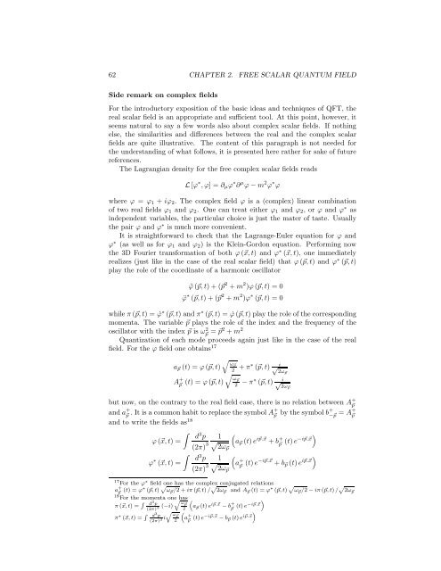
62 CHAPTER 2. FREE SCALAR QUANTUM FIELD
Side remark on complex fields
For the introductory exposition of the basic ideas and techniques of QFT, the
real scalar field is an appropriate and sufficient tool. At this point, however, it
seems natural to say a few words also about complex scalar fields. If nothing
else, the similarities and differences between the real and the complex scalar
fields are quite illustrative. The content of this paragraph is not needed for
the understanding of what follows, it is presented here rather for sake of future
references.
The Lagrangian density for the free complex scalar fields reads
L[ϕ ∗ ,ϕ] = ∂ µ ϕ ∗ ∂ µ ϕ−m 2 ϕ ∗ ϕ
where ϕ = ϕ 1 + iϕ 2 . The complex field ϕ is a (complex) linear combination
of two real fields ϕ 1 and ϕ 2 . One can treat either ϕ 1 and ϕ 2 , or ϕ and ϕ ∗ as
independent variables, the particular choice is just the mater of taste. Usually
the pair ϕ and ϕ ∗ is much more convenient.
It is straightforward to check that the Lagrange-Euler equation for ϕ and
ϕ ∗ (as well as for ϕ 1 and ϕ 2 ) is the Klein-Gordon equation. Performing now
the 3D Fourier transformation of both ϕ(⃗x,t) and ϕ ∗ (⃗x,t), one immediately
realizes (just like in the case of the real scalar field) that ϕ(⃗p,t) and ϕ ∗ (⃗p,t)
play the role of the coordinate of a harmonic oscillator
¨ϕ(⃗p,t)+(⃗p 2 +m 2 )ϕ(⃗p,t) = 0
¨ϕ ∗ (⃗p,t)+(⃗p 2 +m 2 )ϕ ∗ (⃗p,t) = 0
while π(⃗p,t) = ˙ϕ ∗ (⃗p,t) and π ∗ (⃗p,t) = ˙ϕ(⃗p,t) play the role of the corresponding
momenta. The variable ⃗p plays the role of the index and the frequency of the
oscillator with the index ⃗p is ω 2 ⃗p = ⃗p2 +m 2
Quantization of each mode proceeds again just like in the case of the real
field. For the ϕ field one obtains 17
ω⃗p
a ⃗p (t) = ϕ(⃗p,t)√
2 +π∗ i
(⃗p,t) √
2ω⃗p
√
A + ⃗p (t) = ϕ(⃗p,t) ω⃗p
2 −π∗ i
(⃗p,t) √
2ω⃗p
but now, on the contrary to the real field case, there is no relation between A + ⃗p
and a + ⃗p . It is a common habit to replace the symbol A+ ⃗p by the symbol b+ −⃗p = A+ ⃗p
and to write the fields as 18
∫
ϕ(⃗x,t) =
∫
ϕ ∗ (⃗x,t) =
d 3 p
(2π) 3 1
√
2ω⃗p
(
a ⃗p (t)e i⃗p.⃗x +b + ⃗p (t)e−i⃗p.⃗x)
d 3 p 1
(
(2π) 3 √ a + ⃗p (t)e−i⃗p.⃗x +b ⃗p (t)e i⃗p.⃗x)
2ω⃗p
17 For the ϕ ∗ field one has the complex conjugated relations
a + ⃗p (t) = ϕ∗ (⃗p,t) √ ω ⃗p /2+iπ(⃗p,t)/ √ 2ω ⃗p and A ⃗p (t) = ϕ ∗ (⃗p,t) √ ω ⃗p /2−iπ(⃗p,t)/ √ 2ω ⃗p
18 For the momenta one has
π(⃗x,t) = ∫ √
d 3 p ω⃗p
)
(2π) 3 (−i)
(a 2 ⃗p (t)e i⃗p.⃗x −b + ⃗p (t)e−i⃗p.⃗x
π ∗ (⃗x,t) = ∫ √
d 3 p ω⃗p
)
(2π) 3 i
(a + 2 ⃗p (t)e−i⃗p.⃗x −b ⃗p (t)e i⃗p.⃗x