Quantum Field Theory I

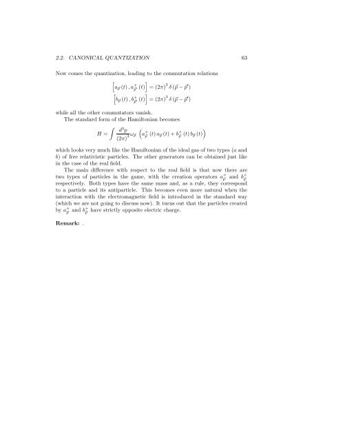
2.2. CANONICAL QUANTIZATION 63
Now comes the quantization, leading to the commutation relations
[ ]
a ⃗p (t),a + ⃗p
(t) = (2π) 3 δ(⃗p−⃗p ′ )
[
′ ]
b ⃗p (t),b + ⃗p
(t) = (2π) 3 δ(⃗p−⃗p ′ )
′
while all the other commutators vanish.
The standard form of the Hamiltonian becomes
∫
d 3 p
(
)
H =
(2π) 3ω ⃗p a + ⃗p (t)a ⃗p(t)+b + ⃗p (t)b ⃗p(t)
which looks very much like the Hamiltonian of the ideal gas of two types (a and
b) of free relativistic particles. The other generators can be obtained just like
in the case of the real field.
The main difference with respect to the real field is that now there are
two types of particles in the game, with the creation operators a + ⃗p and b+ ⃗p
respectively. Both types have the same mass and, as a rule, they correspond
to a particle and its antiparticle. This becomes even more natural when the
interaction with the electromagnetic field is introduced in the standard way
(which we are not going to discuss now). It turns out that the particles created
by a + ⃗p and b+ ⃗p
have strictly opposite electric charge.
Remark: .