Quantum Field Theory I

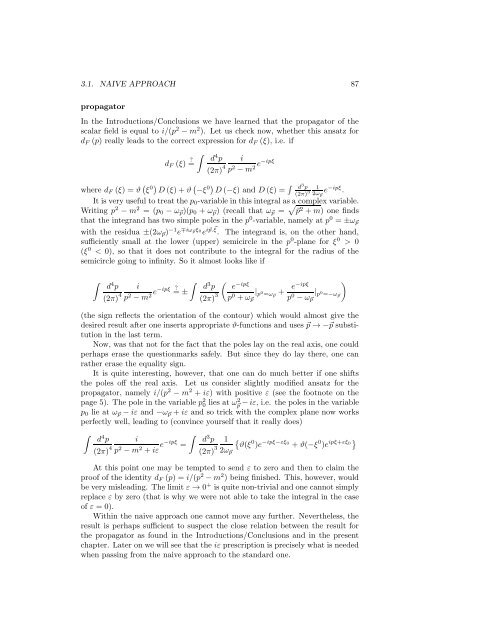
3.1. NAIVE APPROACH 87
propagator
In the Introductions/Conclusions we have learned that the propagator of the
scalar field is equal to i/(p 2 −m 2 ). Let us check now, whether this ansatz for
d F (p) really leads to the correct expression for d F (ξ), i.e. if
∫
d F (ξ) =
d 4 p i
(2π) 4 p 2 −m 2e−ipξ
where d F (ξ) = ϑ ( ξ 0) D(ξ)+ϑ ( −ξ 0) D(−ξ) and D(ξ) = ∫ d 3 p
(2π) 3 1
2ω ⃗p
e −ipξ .
It is very useful to treat the p 0 -variable in this integral asa complex variable.
Writing p 2 − m 2 = (p 0 − ω ⃗p )(p 0 + ω ⃗p ) (recall that ω ⃗p = √ ⃗p 2 +m) one finds
that the integrand has two simple poles in the p 0 -variable, namely at p 0 = ±ω ⃗p
with the residua ±(2ω ⃗p ) −1 e ∓iω ⃗pξ 0
e i⃗p.⃗ξ . The integrand is, on the other hand,
sufficiently small at the lower (upper) semicircle in the p 0 -plane for ξ 0 > 0
(ξ 0 < 0), so that it does not contribute to the integral for the radius of the
semicircle going to infinity. So it almost looks like if
∫
d 4 ∫
p i
= ±
(2π) 4 p 2 −m 2e−ipξ
d 3 ( )
p e
−ipξ
(2π) 3 p 0 | p
+ω 0 =ω ⃗p
+ e−ipξ
⃗p p 0 | p
−ω 0 =−ω ⃗p ⃗p
(the sign reflects the orientation of the contour) which would almost give the
desired result after one inserts appropriate ϑ-functions and uses ⃗p → −⃗p substitution
in the last term.
Now, was that not for the fact that the poles lay on the real axis, one could
perhaps erase the questionmarks safely. But since they do lay there, one can
rather erase the equality sign.
It is quite interesting, however, that one can do much better if one shifts
the poles off the real axis. Let us consider slightly modified ansatz for the
propagator, namely i/(p 2 − m 2 + iε) with positive ε (see the footnote on the
page 5). The pole in the variable p 2 0 lies at ω2 ⃗p
−iε, i.e. the poles in the variable
p 0 lie at ω ⃗p −iε and −ω ⃗p +iε and so trick with the complex plane now works
perfectly well, leading to (convince yourself that it really does)
∫
d 4 ∫
p i
(2π) 4 p 2 −m 2 +iε e−ipξ =
d 3 p 1 {
ϑ(ξ 0
(2π) 3 )e −ipξ−εξ0 +ϑ(−ξ 0 )e ipξ+εξ0}
2ω ⃗p
At this point one may be tempted to send ε to zero and then to claim the
proof of the identity d F (p) = i/(p 2 −m 2 ) being finished. This, however, would
be very misleading. The limit ε → 0 + is quite non-trivial and one cannot simply
replace ε by zero (that is why we were not able to take the integral in the case
of ε = 0).
Within the naive approach one cannot move any further. Nevertheless, the
result is perhaps sufficient to suspect the close relation between the result for
the propagator as found in the Introductions/Conclusions and in the present
chapter. Later on we will see that the iε prescription is precisely what is needed
when passing from the naive approach to the standard one.