Quantum Field Theory I

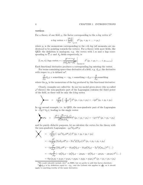
4 CHAPTER 1. INTRODUCTIONS
vertices
For a theory of one field ϕ, the factor corresponding to the n-leg vertex is 3
n-leg vertex = i ∂n L
∂ϕ n ∣
∣∣∣ϕ=0
δ 4 (p 1 +p 2 +...+p n )
where p i is the momentum corresponding to the i-th leg (all momenta are understood
to be pointing towards the vertex). For a theory with more fields, like
QED, the definition is analogous, e.g. the vertex with l,m and n legs corresponding
to ψ,ψ and A µ -fields respectively, is
(l,m,n)-legs vertex = i
∂ l+m+n L
∂A l µ∂ψ m ∂ψ n ∣
∣∣∣∣fields=0
δ 4 (p 1 +p 2 +...+p l+m+n )
Each functional derivative produces a corresponding leg entering the vertex.
For terms containing space-time derivative of a field, e.g. ∂ µ ϕ, the derivative
with respec to ϕ is defined as 4
∂
∂ϕ ∂ µϕ×something = −ip µ ×something+∂ µ ϕ× ∂
∂ϕ something
where the p µ is the momentum of the leg produced by this functional derivative.
Clearly, examples are called for. In our toy-model given above (the so-called
ϕ 3 -theory) the non-quadratic part of the Lagrangian contains the third power
of the field, so there will be only the 3-leg vertex
¡=i ∂3
∂ϕ 3 (
− g 3! ϕ3) δ 4 (p 1 +p 2 +p 3 ) = −igδ 4 (p 1 +p 2 +p 3 )
In our second example, i.e. in QED, the non-quadratic part of the Lagrangian
is −ψqγ µ A µ ψ, leading to the single vertex
¡=i ∂3( −qψγ µ A µ ψ )
∂ψ∂ψ∂A µ
δ 4 (p 1 +p 2 +p 3 ) = −iqγ µ δ 4 (p 1 +p 2 +p 3 )
and for purely didactic purposes, let us calculate the vertex for the theory with
the non-quadratic Lagrangian −gϕ 2 ∂ µ ϕ∂ µ ϕ
¡=i ∂4
∂ϕ 4 (
−gϕ 2 ∂ µ ϕ∂ µ ϕ ) δ 4 (p 1 +p 2 +p 3 +p 4 )
= −ig ∂3 (
2ϕ∂µ
∂ϕ 3 ϕ∂ µ ϕ−2iϕ 2 p µ 1 ∂ µϕ ) δ 4 (p 1 +p 2 +p 3 +p 4 )
= −ig ∂2 (
2∂µ
∂ϕ 2 ϕ∂ µ ϕ−4iϕp µ 2 ∂ µϕ−4iϕp µ 1 ∂ µϕ−2ϕ 2 p µ 1 p )
2,µ δ 4 (...)
= −i4g ∂
∂ϕ (−ipµ 3 ∂ µϕ−ip µ 2 ∂ µϕ−ϕp 2 p 3 −ip µ 1 ∂ µϕ−ϕp 1 p 3 −ϕp 1 p 2 )δ 4 (...)
= 4ig(p 1 p 2 +p 1 p 3 +p 1 p 4 +p 2 p 3 +p 2 p 4 +p 3 p 4 )δ 4 (p 1 +p 2 +p 3 +p 4 )
3 We could (should) include (2π) 4 on RHS, but we prefer to add this factor elsewhere.
4 ∂
∂
∂µϕ is by definition equal to −ipµ, and the Leibniz rule applies to , as it should
∂ϕ ∂ϕ
apply to anything worthy of the name derivative.