Quantum Field Theory I

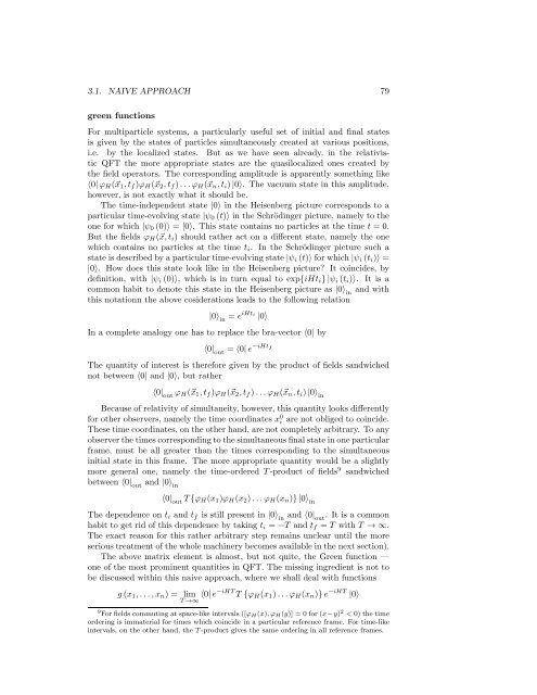
3.1. NAIVE APPROACH 79
green functions
For multiparticle systems, a particularly useful set of initial and final states
is given by the states of particles simultaneously created at various positions,
i.e. by the localized states. But as we have seen already, in the relativistic
QFT the more appropriate states are the quasilocalized ones created by
the field operators. The corresponding amplitude is apparently something like
〈0|ϕ H (⃗x 1 ,t f )ϕ H (⃗x 2 ,t f )...ϕ H (⃗x n ,t i )|0〉. The vacuum state in this amplitude,
however, is not exactly what it should be.
The time-independent state |0〉 in the Heisenberg picture corresponds to a
particular time-evolving state |ψ 0 (t)〉 in the Schrödinger picture, namely to the
one for which |ψ 0 (0)〉 = |0〉. This state contains no particles at the time t = 0.
But the fields ϕ H (⃗x,t i ) should rather act on a different state, namely the one
which contains no particles at the time t i . In the Schrödinger picture such a
state is described byaparticulartime-evolvingstate|ψ i (t)〉 forwhich |ψ i (t i )〉 =
|0〉. How does this state look like in the Heisenberg picture It coincides, by
definition, with |ψ i (0)〉, which is in turn equal to exp{iHt i }|ψ i (t i )〉. It is a
common habit to denote this state in the Heisenberg picture as |0〉 in
and with
this notationn the above cosiderations leads to the following relation
|0〉 in
= e iHti |0〉
In a complete analogy one has to replace the bra-vector 〈0| by
〈0| out
= 〈0|e −iHt f
The quantity of interest is therefore given by the product of fields sandwiched
not between 〈0| and |0〉, but rather
〈0| out
ϕ H (⃗x 1 ,t f )ϕ H (⃗x 2 ,t f )...ϕ H (⃗x n ,t i )|0〉 in
Because of relativity of simultaneity, however, this quantity looks differently
for other observers, namely the time coordinates x 0 i are not obliged to coincide.
These time coordinates, on the other hand, are not completely arbitrary. To any
observerthetimescorrespondingtothesimultaneousfinalstateinoneparticular
frame, must be all greater than the times corresponding to the simultaneous
initial state in this frame. The more appropriate quantity would be a slightly
more general one, namely the time-ordered T-product of fields 9 sandwiched
between 〈0| out
and |0〉 in
〈0| out
T{ϕ H (x 1 )ϕ H (x 2 )...ϕ H (x n )}|0〉 in
The dependence on t i and t f is still present in |0〉 in
and 〈0| out
. It is a common
habit to get rid of this dependence by taking t i = −T and t f = T with T → ∞.
The exact reason for this rather arbitrary step remains unclear until the more
serioustreatment ofthe wholemachinerybecomes availablein the next section).
The above matrix element is almost, but not quite, the Green function —
one of the most prominent quantities in QFT. The missing ingredient is not to
be discussed within this naive approach, where we shall deal with functions
g(x 1 ,...,x n ) = lim
T→∞ 〈0|e−iHT T {ϕ H (x 1 )...ϕ H (x n )}e −iHT |0〉
9 For fields commuting at space-like intervals ([ϕ H (x),ϕ H (y)] = 0 for (x−y) 2 < 0) the time
ordering is immaterial for times which coincide in a particular reference frame. For time-like
intervals, on the other hand, the T-product gives the same ordering in all reference frames.