Quantum Field Theory I

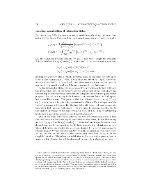
74 CHAPTER 3. INTERACTING QUANTUM FIELDS
canonical quantization of interacting fields
For interacting fields the quantization proceeds basically along the same lines
as for the free fields. Fields and the conjugated momenta are Fourier expanded
∫
d 3 p 1
(
ϕ(⃗x,t) =
(2π) 3 √ a ⃗p (t)e i⃗p.⃗x +a + ⃗p (t)e−i⃗p.⃗x)
2ω⃗p
∫ √
d 3 p ω⃗p
π(⃗x,t) = −i
(a
(2π) 3 ⃗p (t)e i⃗p.⃗x −a + ⃗p
2
(t)e−i⃗p.⃗x)
and the canonical Poisson brackets for ϕ(⃗x,t) and π(⃗x,t) imply the standard
Poisson brackets for a ⃗p (t) and a + ⃗p ′ (t) which lead to the commutation relations
[a ⃗p (t),a + ⃗p ′ (t)] = (2π) 3 δ(⃗p−⃗p ′ )
[a ⃗p (t),a ⃗p ′ (t)] = [a + ⃗p (t),a+ ⃗p ′ (t)] = 0.
holding for arbitrary time t (which, however, must be the same for both operators
in the commutator — that is why they are known as ”equal-time commutation
relations”). At any fixed time, these commutation relations can be
represented by creation and annihilation operators in the Fock space.
So far, it looks like if there is no serious difference between the free fields and
the interacting ones. In the former case the appearence of the Fock space was
the last important step which enabled us to complete the canonicalquantization
program. For the interacting fields, however, one does not have the Fock space,
but rather Fock spaces. The point is that for different times t the a + ⃗p
(t) and
a ⃗p ′ (t) operators are, in principle, represented in different Fock subspaces of the
”large” non-separable space. For the free fields all these Fock spaces coincide,
they are in fact just one Fock space — we were able to demonstrate this due to
the explicit knowledge of the time evolution of a + ⃗p and a ⃗p ′. But for interacting
fields such a knowledge is not at our disposal anymore 3 .
One of the main differences between the free and interacting fields is that
the time evolution becomes highly nontrivial for the latter. In the Heisenberg
picture,theequationsfora ⃗p (t)anda + ⃗p
(t)donotleadtoasimpleharmonictimedependence,
nor do the equations for the basis states in the Schrödingerpicture.
′
These difficulties are evaded (to a certain degree) by a clever approximative
scheme, namely by the perturbation theory in the so-called interaction picture.
In this section, we will develop the scheme and learn how to use it in the
simplified version. The scheme is valid also in the standard approach, but its
usage is a bit different (as will be discussed thoroughly in the next section).
3 Not only one cannot prove for the interacting fields that the Fock spaces for a + (t) and ⃗p
a ⃗p ′ (t) at different times coincide, one can even prove the opposite, namely that these Fock
spaces are, as a rule, different subspaces of the ”large” non-separable space. This means that,
strictly speaking, one cannot avoid the mathematics of the non-separable linear spaces when
dealing with interacting fields. We will, nevertheless, try to ignore all the difficulties related
to non-separability as long as possible. This applies to the present naive approach as well as
to the following standard approach. We will return to these difficulties only in the subsequent
section devoted again to ”contemplations and subtleties”.