Quantum Field Theory I

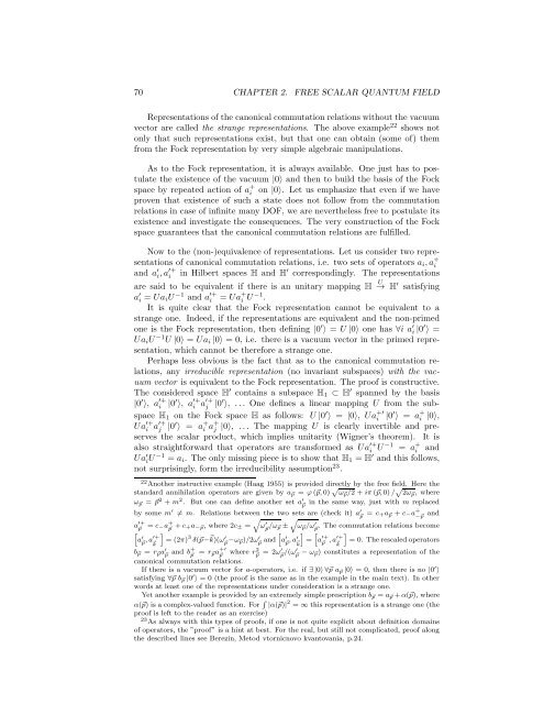
70 CHAPTER 2. FREE SCALAR QUANTUM FIELD
Representations of the canonical commutation relations without the vacuum
vector are called the strange representations. The above example 22 shows not
only that such representations exist, but that one can obtain (some of) them
from the Fock representation by very simple algebraic manipulations.
As to the Fock representation, it is always available. One just has to postulate
the existence of the vacuum |0〉 and then to build the basis of the Fock
space by repeated action of a + i on |0〉. Let us emphasize that even if we have
proven that existence of such a state does not follow from the commutation
relations in case of infinite many DOF, we are nevertheless free to postulate its
existence and investigate the consequences. The very construction of the Fock
space guarantees that the canonical commutation relations are fulfilled.
Now to the (non-)equivalence of representations. Let us consider two representations
of canonical commutation relations, i.e. two sets of operators a i ,a + i
and a ′ i ,a′+ i in Hilbert spaces H and H ′ correspondingly. The representations
are said to be equivalent if there is an unitary mapping H → U H ′ satisfying
a ′ i = Ua iU −1 and a ′+
i = Ua + i U−1 .
It is quite clear that the Fock representation cannot be equivalent to a
strange one. Indeed, if the representations are equivalent and the non-primed
one is the Fock representation, then defining |0 ′ 〉 = U |0〉 one has ∀i a ′ i |0′ 〉 =
Ua i U −1 U |0〉 = Ua i |0〉 = 0, i.e. there is a vacuum vector in the primed representation,
which cannot be therefore a strange one.
Perhaps less obvious is the fact that as to the canonical commutation relations,
any irreducible representation (no invariant subspaces) with the vacuum
vector is equivalent to the Fock representation. The proof is constructive.
The considered space H ′ contains a subspace H 1 ⊂ H ′ spanned by the basis
|0 ′ 〉, a ′+
i |0 ′ 〉, a ′+
i a ′+
j |0 ′ 〉, ... One defines a linear mapping U from the subspace
H 1 on the Fock space H as follows: U |0 ′ 〉 = |0〉, Ua +′
i |0 ′ 〉 = a + i |0〉,
Ua ′+
i a ′+
j |0 ′ 〉 = a + i a+ j |0〉, ... The mapping U is clearly invertible and preserves
the scalar product, which implies unitarity (Wigner’s theorem). It is
also straightforward that operators are transformed as Ua ′+
i U −1 = a + i and
Ua ′ i U−1 = a i . The only missing piece is to show that H 1 = H ′ and this follows,
not surprisingly, form the irreducibility assumption 23 .
22 Another instructive example (Haag 1955) is provided directly by the free field. Here the
standard annihilation operators are given by a ⃗p = ϕ(⃗p,0) √ ω ⃗p /2 + iπ(⃗p,0)/ √ 2ω ⃗p , where
ω ⃗p = ⃗p 2 + m 2 . But one can define another set a ′ in the same way, just with m replaced
⃗p
by some m ′ ≠ m. Relations between the two sets are (check it) a ′ ⃗p = c +a ⃗p + c − a + √ √
−⃗p and
a ′+
⃗p = c −a + ⃗p +c +a −⃗p , where 2c ± = ω ⃗p ′/ω ⃗p ± ω ⃗p /ω ⃗p ′ . The commutation relations become
[ ]
a ′ ⃗p ,a′+ = (2π) 3 δ(⃗p− ⃗ [ ] [ ]
k)(ω ⃗ ′ k ⃗p −ω ⃗p)/2ω ⃗p ′ and a ′ ⃗p ,a′ = a ′+
⃗ k ⃗p ,a′+ = 0. The rescaled operators
⃗ k
b ⃗p = r ⃗p a ′ ⃗p and b+ ⃗p = r ⃗pa +′ where r ⃗p ⃗p 2 = 2ω′ ⃗p /(ω′ ⃗p − ω ⃗p) constitutes a representation of the
canonical commutation relations.
If there is a vacuum vector for a-operators, i.e. if ∃|0〉∀⃗p a ⃗p |0〉 = 0, then there is no |0 ′ 〉
satisfying ∀⃗p b ⃗p |0 ′ 〉 = 0 (the proof is the same as in the example in the main text). In other
words at least one of the representations under consideration is a strange one.
Yet another example is provided by an extremely simple prescription b ⃗p = a ⃗p +α(⃗p), where
α(⃗p) is a complex-valued function. For ∫ |α(⃗p)| 2 = ∞ this representation is a strange one (the
proof is left to the reader as an exercise)
23 As always with this types of proofs, if one is not quite explicit about definition domains
of operators, the ”proof” is a hint at best. For the real, but still not complicated, proof along
the described lines see Berezin, Metod vtornicnovo kvantovania, p.24.