Quantum Field Theory I

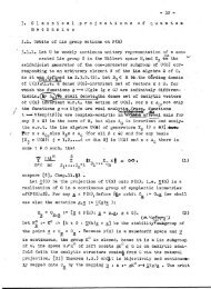
1.2. MANY-BODY QUANTUM MECHANICS 31
1.2.4 The bird’s-eye view of the solid state physics
Even if we are not going to entertain ourselves with calculations within the
creation and annihilation operatorsformalism of the non-relativistic many-body
QM, we may still want to spend some time on formulation of a specific example.
The reason is that the example may turn out to be quite instructive. This,
however, is not guaranteed. Moreover,the content ofthis section is not requisite
for the rest of the text. The reader is therefore encouraged to skip the section
in the first (and perhaps also in any subsequent) reading.
The basic approximations of the solid state physics
∆ i
2M −∑ ∆ j
j
∑
8π i≠j
A solid state physics deals with a macroscopic number of nuclei and electrons,
interacting electromagnetically. The dominant interaction is the Coulomb one,
responsible for the vast majority of solid state phenomena covering almost everything
except of magnetic properties. For one type of nucleus with the proton
number Z (generalization is straightforward) the Hamiltonian in the wavefunction
formalism 37 is H = − ∑ i
U( R) ⃗ = 1 ∑
Z 2 e 2
8π i≠j | R ⃗ i−R ⃗ , V(⃗r) = 1
j|
and (obviously) R ⃗ = ( R ⃗ 1 ,...), ⃗r = (⃗r 1 ,...). If desired, more than Coulomb can
be accounted for by changing U, V and W appropriately.
Although looking quite innocent, this Hamiltonian is by far too difficult to
calculate physical properties of solids directly from it. Actually, no one has ever
succeeded in proving even the basic experimental fact, namely that nuclei in
solids build a lattice. Therefore, any attempt to grasp the solid state physics
theoretically, starts from the series of clever approximations.
The first one is the Born-Oppenheimer adiabatic approximation which enables
us to treat electrons and nuclei separately. The second one is the Hartree-
Fockapproximation,whichenablesustoreducetheunmanageablemany-electron
problem to a manageable single-electron problem. Finally, the third of the
celebrated approximations is the harmonic approximation, which enables the
explicit (approximate) solution of the nucleus problem.
These approximations are used in many areas of quantum physics, let us
mention the QM of molecules as a prominent example. There is, however, an
important difference between the use of the approximations for molecules and
for solids. The difference is in the number of particles involved (few nuclei
and something like ten times more electrons in molecules, Avogadro number
in solids). So while in the QM of molecules, one indeed solves the equations
resulting from the individual approximations, in case of solids one (usually)
does not. Here the approximations are used mainly to setup the conceptual
framework for both theoretical analysis and experimental data interpretation.
In neither of the three approximations the Fock space formalism is of any
great help (although for the harmonic approximation, the outcome is often formulated
in this formalism). But when movingbeyondthe three approximations,
this formalism is by far the most natural and convenient one.
2m +U(⃗ R)+V(⃗r)+W( R,⃗r), ⃗ where
e 2
|⃗r , W(⃗ i−⃗r j|
R,⃗r) = − 1 ∑
Ze 2
8π i,j | R ⃗ i−⃗r j|
37 If required, it is quite straightforward (even if not that much rewarding) to rewrite
the Hamiltonian in terms of the creation and annihilation operators (denoted as uppercase
and lowercase for nuclei and electrons respectively) H = ∫ ( )
d 3 p p
2
2M A+ ⃗p A ⃗p + p2
2m a+ ⃗p a ⃗p +
e 2 ∫ )
8π d 3 x d 3 1
y
(Z 2 A + |⃗x−⃗y| ⃗x A+ ⃗y A ⃗yA ⃗x −ZA + ⃗x a+ ⃗y a ⃗yA ⃗x +a + ⃗x a+ ⃗y a ⃗ya ⃗x .