SAWE Report - Cal Poly San Luis Obispo

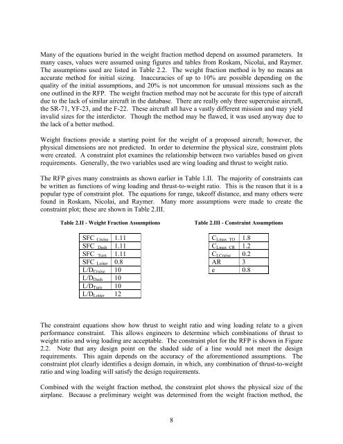
Many of the equations buried in the weight fraction method depend on assumed parameters. In
many cases, values were assumed using figures and tables from Roskam, Nicolai, and Raymer.
The assumptions used are listed in Table 2.2. The weight fraction method is by no means an
accurate method for initial sizing. Inaccuracies of up to 10% are possible depending on the
quality of the initial assumptions, and 20% is not uncommon for unusual missions such as the
one outlined in the RFP. The weight fraction method may not be accurate for this type of aircraft
due to the lack of similar aircraft in the database. There are really only three supercruise aircraft,
the SR-71, YF-23, and the F-22. These aircraft all have a vastly different mission and may yield
invalid sizes for the interdictor. Though the method may be flawed, it was used anyway due to
the lack of a better method.
Weight fractions provide a starting point for the weight of a proposed aircraft; however, the
physical dimensions are not predicted. In order to determine the physical size, constraint plots
were created. A constraint plot examines the relationship between two variables based on given
requirements. Generally, the two variables used are wing loading and thrust to weight ratio.
The RFP gives many constraints as shown earlier in Table 1.II. The majority of constraints can
be written as functions of wing loading and thrust-to-weight ratio. This is the reason that it is a
popular type of constraint plot. The equations for range, takeoff distance, and many others were
found in Roskam, Nicolai, and Raymer. Many more assumptions were made to create the
constraint plot; these are shown in Table 2.III.
Table 2.II - Weight Fraction Assumptions
SFC _Cruise 1.11
SFC _Dash 1.11
SFC _Turn 1.11
SFC _Loiter 0.8
L/D Cruise 10
L/D Dash 10
L/D Turn 10
L/D Loiter 12
Table 2.III - Constraint Assumptions
C Lmax_TO 1.8
C Lmax_CR 1.2
C LCruise 0.2
AR 3
e 0.8
The constraint equations show how thrust to weight ratio and wing loading relate to a given
performance constraint. This allows engineers to determine which combinations of thrust to
weight ratio and wing loading are acceptable. The constraint plot for the RFP is shown in Figure
2.2. Note that any design point on the shaded side of a line would not meet the design
requirements. This again depends on the accuracy of the aforementioned assumptions. The
constraint plot clearly identifies a design domain, in which, any combination of thrust-to-weight
ratio and wing loading will satisfy the design requirements.
Combined with the weight fraction method, the constraint plot shows the physical size of the
airplane. Because a preliminary weight was determined from the weight fraction method, the
8