Applied Superconductivity - Walther Meißner Institut - Bayerische ...

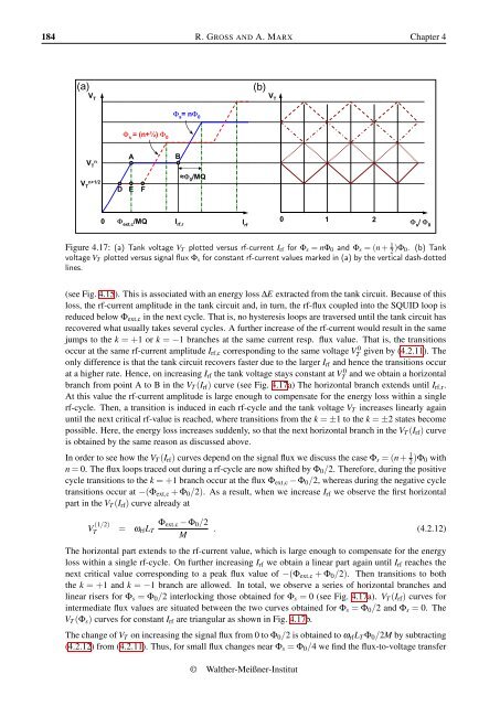
184 R. GROSS AND A. MARX Chapter 4(a)(b)V TV TA BΦ s= (n+½) Φ 0Φ s= nΦ 0V TnV Tn+1/2D E F≈Φ 0/MQ0 Φ ext,c/MQ0 1 2I rf,rI rfΦ s/ Φ 0Figure 4.17: (a) Tank voltage V T plotted versus rf-current I rf for Φ s = nΦ 0 and Φ s = (n + 1 2 )Φ 0. (b) Tankvoltage V T plotted versus signal flux Φ s for constant rf-current values marked in (a) by the vertical dash-dottedlines.(see Fig. 4.15). This is associated with an energy loss ∆E extracted from the tank circuit. Because of thisloss, the rf-current amplitude in the tank circuit and, in turn, the rf-flux coupled into the SQUID loop isreduced below Φ ext,c in the next cycle. That is, no hysteresis loops are traversed until the tank circuit hasrecovered what usually takes several cycles. A further increase of the rf-current would result in the samejumps to the k = +1 or k = −1 branches at the same current resp. flux value. That is, the transitionsoccur at the same rf-current amplitude I rf,c corresponding to the same voltage VT 0 given by (4.2.11). Theonly difference is that the tank circuit recovers faster due to the larger I rf and hence the transitions occurat a higher rate. Hence, on increasing I rf the tank voltage stays constant at VT 0 and we obtain a horizontalbranch from point A to B in the V T (I rf ) curve (see Fig. 4.17a) The horizontal branch extends until I rf,r .At this value the rf-current amplitude is large enough to compensate for the energy loss within a singlerf-cycle. Then, a transition is induced in each rf-cycle and the tank voltage V T increases linearly againuntil the next critical rf-value is reached, where transitions from the k = ±1 to the k = ±2 states becomepossible. Here, the energy loss increases suddenly, so that the next horizontal branch in the V T (I rf ) curveis obtained by the same reason as discussed above.In order to see how the V T (I rf ) curves depend on the signal flux we discuss the case Φ s = (n+ 1 2 )Φ 0 withn = 0. The flux loops traced out during a rf-cycle are now shifted by Φ 0 /2. Therefore, during the positivecycle transitions to the k = +1 branch occur at the flux Φ ext,c − Φ 0 /2, whereas during the negative cycletransitions occur at −(Φ ext,c + Φ 0 /2). As a result, when we increase I rf we observe the first horizontalpart in the V T (I rf ) curve already atV (1/2)T = ω rf L TΦ ext,c − Φ 0 /2M. (4.2.12)The horizontal part extends to the rf-current value, which is large enough to compensate for the energyloss within a single rf-cycle. On further increasing I rf we obtain a linear part again until I rf reaches thenext critical value corresponding to a peak flux value of −(Φ ext,c + Φ 0 /2). Then transitions to boththe k = +1 and k = −1 branch are allowed. In total, we observe a series of horizontal branches andlinear risers for Φ s = Φ 0 /2 interlocking those obtained for Φ s = 0 (see Fig. 4.17a). V T (I rf ) curves forintermediate flux values are situated between the two curves obtained for Φ s = Φ 0 /2 and Φ s = 0. TheV T (Φ s ) curves for constant I rf are triangular as shown in Fig. 4.17b.The change of V T on increasing the signal flux from 0 to Φ 0 /2 is obtained to ω rf L T Φ 0 /2M by subtracting(4.2.12) from (4.2.11). Thus, for small flux changes near Φ s = Φ 0 /4 we find the flux-to-voltage transfer© Walther-Meißner-Institut