Measurement of the Jet Energy Scale in the CMS experiment ... - IIHE
Measurement of the Jet Energy Scale in the CMS experiment ... - IIHE
Measurement of the Jet Energy Scale in the CMS experiment ... - IIHE

You also want an ePaper? Increase the reach of your titles
YUMPU automatically turns print PDFs into web optimized ePapers that Google loves.
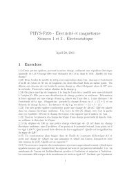
CHAPTER 5: Estimat<strong>in</strong>g <strong>of</strong> <strong>the</strong> <strong>Jet</strong> <strong>Energy</strong> <strong>Scale</strong> Calibration Factor 123#Events1008060tt+jets semi-ele (146.8 entries)tt+jets o<strong>the</strong>r (23.4 entries)S<strong>in</strong>gleTop+jets (7.5 entries)Z+jets (3.5 entries)W+jets (15.1 entries)QCD (4.6 entries)Data (36.1 pb-1) (176.0 entries)#Events2101040120-1100 0.2 0.4 0.6 0.8 1max Probability <strong>of</strong> <strong>the</strong> K<strong>in</strong>Fit0 0.2 0.4 0.6 0.8 1max Probability <strong>of</strong> <strong>the</strong> K<strong>in</strong>FitFigure 5.34: The distribution <strong>of</strong> <strong>the</strong> maximum probability returned by <strong>the</strong> k<strong>in</strong>ematicfit shown <strong>in</strong> normal scale (left) and logarithmic scale (right). The collision data eventsare overimposed to <strong>the</strong> simulation for comparison purpose.one may expect to obta<strong>in</strong> a number <strong>of</strong> e+jets t¯t events which survive <strong>the</strong> PK<strong>in</strong>Fit max tobe about 36.1 × 75 ∼ 27, given that <strong>the</strong> same event selection cuts are applied. As it100can be seen from Table 5.16, <strong>the</strong>re are about 42 e+jets t¯t events rema<strong>in</strong>ed at <strong>the</strong> samelevel <strong>of</strong> <strong>the</strong> selection procedure, hence more events than what is expected. This canbe expla<strong>in</strong>ed s<strong>in</strong>ce a looser set <strong>of</strong> cuts has been applied on <strong>the</strong> reconstructed jets whenrunn<strong>in</strong>g on <strong>the</strong> data.With <strong>the</strong> 34 events <strong>in</strong> <strong>the</strong> collision data pass<strong>in</strong>g <strong>the</strong> full event selection, one can startestimat<strong>in</strong>g <strong>the</strong> residual light and b jet energy correction factors. For each <strong>of</strong> <strong>the</strong> surviveddata events, <strong>the</strong> twoi-dimensional grid <strong>of</strong> po<strong>in</strong>ts which is filled with <strong>the</strong> k<strong>in</strong>ematicfit probabilities, P K<strong>in</strong>Fit (∆E l , ∆E b ), is transformed to a χ 2 denoted as χ 2 (∆E l , ∆E b ).The χ 2 values <strong>in</strong> each po<strong>in</strong>t <strong>of</strong> <strong>the</strong> grid are summed for all <strong>of</strong> <strong>the</strong> f<strong>in</strong>al selected dataevents. The results can be found <strong>in</strong> Figure 5.35.The f<strong>in</strong>al estimated light and b jet energy corrections are determ<strong>in</strong>ed at <strong>the</strong> m<strong>in</strong>imumpo<strong>in</strong>t <strong>of</strong> <strong>the</strong> χ 2 (∆E l , ∆E b ) distribution which is shown <strong>in</strong> Figure 5.35. Theprojected χ 2 distribution <strong>in</strong> <strong>the</strong> direction <strong>of</strong> <strong>the</strong> ∆E l and ∆E b , shown <strong>in</strong> Figure 5.36,are fitted with a second-degree polynomial and <strong>the</strong> po<strong>in</strong>ts with <strong>the</strong> m<strong>in</strong>imum valuesare quoted as <strong>the</strong> light and b jet energy calibration factors, respectively. The f<strong>in</strong>alestimated residual jet energy corrections, which are obta<strong>in</strong>ed us<strong>in</strong>g <strong>the</strong> 36.1pb −1 <strong>of</strong> <strong>the</strong>accumulated collision data, are listed <strong>in</strong> Table 5.17.In order to compare <strong>the</strong> results derived from <strong>the</strong> collision data events with <strong>the</strong> resultsobta<strong>in</strong>ed from <strong>the</strong> simulation, <strong>the</strong> same procedure to determ<strong>in</strong>e <strong>the</strong> residual jetenergy corrections can be applied us<strong>in</strong>g only <strong>the</strong> f<strong>in</strong>al survived simulated events whichare listed <strong>in</strong> Table 5.16. The results <strong>of</strong> <strong>the</strong> residual jet energy corrections estimatedbased on <strong>the</strong> simulation are also shown <strong>in</strong> Table 5.17.It should be noted that <strong>the</strong> statistical uncerta<strong>in</strong>ties on <strong>the</strong> estimated jet energy correctionslisted <strong>in</strong> Table 5.17, are corrected for <strong>the</strong> non-unity width <strong>of</strong> <strong>the</strong> pull distributions.The systematical uncerta<strong>in</strong>ties on <strong>the</strong> estimated residual light and b jet energy correctionsderived from <strong>the</strong> simulation are also quoted. Clearly <strong>the</strong> uncerta<strong>in</strong>ties on <strong>the</strong>estimated results are dom<strong>in</strong>ated by <strong>the</strong> statistics. The statistical uncerta<strong>in</strong>ties can be