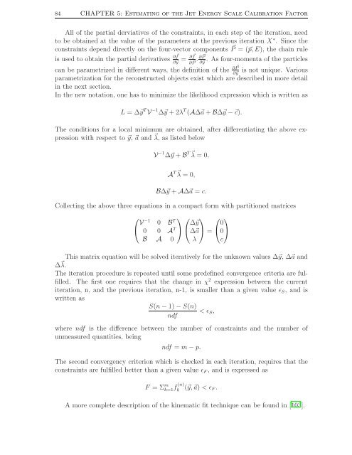
84 CHAPTER 5: Estimat<strong>in</strong>g <strong>of</strong> <strong>the</strong> <strong>Jet</strong> <strong>Energy</strong> <strong>Scale</strong> Calibration FactorAll <strong>of</strong> <strong>the</strong> partial derviatives <strong>of</strong> <strong>the</strong> constra<strong>in</strong>ts, <strong>in</strong> each step <strong>of</strong> <strong>the</strong> iteration, needto be obta<strong>in</strong>ed at <strong>the</strong> value <strong>of</strong> <strong>the</strong> parameters at <strong>the</strong> previous iteration X ∗ . S<strong>in</strong>ce <strong>the</strong>constra<strong>in</strong>ts depend directly on <strong>the</strong> four-vector components P ⃗ = (⃗p, E), <strong>the</strong> cha<strong>in</strong> ruleis used to obta<strong>in</strong> <strong>the</strong> partial derivatives ∂ f ⃗ = ∂ f ⃗∂⃗y ∂ ⃗P .∂ P ⃗ . As four-momenta <strong>of</strong> <strong>the</strong> particles∂⃗ycan be parametrized <strong>in</strong> different ways, <strong>the</strong> def<strong>in</strong>ition <strong>of</strong> <strong>the</strong> ∂ P ⃗ is not unique. Various∂⃗yparametrization for <strong>the</strong> reconstructed objects exist which are described <strong>in</strong> more detail<strong>in</strong> <strong>the</strong> next section.In <strong>the</strong> new notation, one has to m<strong>in</strong>imize <strong>the</strong> likelihood expression which is written asL = ∆⃗y T V −1 ∆⃗y + 2λ T (A∆⃗a + B∆⃗y −⃗c).The conditions for a local m<strong>in</strong>imum are obta<strong>in</strong>ed, after differentiat<strong>in</strong>g <strong>the</strong> above expressionwith respect to ⃗y, ⃗a and ⃗ λ, as listed belowV −1 ∆⃗y + B T ⃗ λ = 0,A T ⃗ λ = 0,B∆⃗y + A∆⃗a = c.Collect<strong>in</strong>g <strong>the</strong> above three equations <strong>in</strong> a compact form with partitioned matrices⎛ ⎞ ⎛ ⎞ ⎛ ⎞V −1 0 B T ∆⃗y 0⎝ 0 0 A T ⎠ ⎝∆⃗a⎠ = ⎝0⎠B A 0 λ cThis matrix equation will be solved iteratively for <strong>the</strong> unknown values ∆⃗y, ∆⃗a and∆ ⃗ λ.The iteration procedure is repeated until some predef<strong>in</strong>ed convergence criteria are fulfilled.The first one requires that <strong>the</strong> change <strong>in</strong> χ 2 expression between <strong>the</strong> currentiteration, n, and <strong>the</strong> previous iteration, n-1, is smaller than a given value ǫ S , and iswritten asS(n − 1) − S(n)< ǫ S ,ndfwhere ndf is <strong>the</strong> difference between <strong>the</strong> number <strong>of</strong> constra<strong>in</strong>ts and <strong>the</strong> number <strong>of</strong>unmeasured quantities, be<strong>in</strong>gndf = m − p.The second convergency criterion which is checked <strong>in</strong> each iteration, requires that <strong>the</strong>constra<strong>in</strong>ts are fulfilled better than a given value ǫ F , and is expressed asF = Σ m k=1 f(n) k(⃗y,⃗a) < ǫ F .A more complete description <strong>of</strong> <strong>the</strong> k<strong>in</strong>ematic fit technique can be found <strong>in</strong> [103].
CHAPTER 5: Estimat<strong>in</strong>g <strong>of</strong> <strong>the</strong> <strong>Jet</strong> <strong>Energy</strong> <strong>Scale</strong> Calibration Factor 855.2.2 Four-Vector ParametrizationSeveral parametrizations <strong>in</strong> <strong>the</strong> k<strong>in</strong>ematic fit package are implemented, two <strong>of</strong> whichare commonly used <strong>in</strong> hadron colliders and are <strong>in</strong>troduced briefly here. A first one,called TFitParticleEtThetaPhi, uses E T , θ and φ variables for parametrization. Themomentum vector and <strong>the</strong> energy can be written <strong>in</strong> this parametrization as⎛ ⎞E T cosφ⃗p f = ⎝E T s<strong>in</strong> φ⎠ ,E T cot θE = E Ts<strong>in</strong> θ .In a second parametrization, called TFitParticleEtEtaPhi, where E T , η and φ variablesare used as parameters, <strong>the</strong> four-vector can be expressed as⎛ ⎞E T cosφ⃗p f = ⎝ E T s<strong>in</strong> φ ⎠,E T s<strong>in</strong>h ηE = E T cosh η.In <strong>the</strong> two parametrizations expla<strong>in</strong>ed above, <strong>the</strong> objects are considered as massless.In this study, TFitParticleEtThetaPhi parametrization is used with an additionalrequirement. Dur<strong>in</strong>g <strong>the</strong> fit procedure, it is crucial to keep <strong>the</strong> ratio <strong>of</strong> <strong>the</strong> measuredenergy <strong>of</strong> a jet to its measured momentum constant. Hence, <strong>in</strong> <strong>the</strong> k<strong>in</strong>ematic fit methodwhich is used <strong>in</strong> <strong>the</strong> current study, this additional requirement is applied which isexpressed as followsE fitted|⃗p fitted | = E measured|⃗p measured | .5.2.3 Resolutions on <strong>the</strong> <strong>Jet</strong> K<strong>in</strong>ematicsThe uncerta<strong>in</strong>ties on <strong>the</strong> measured parameters enter <strong>the</strong> k<strong>in</strong>ematic fit package via <strong>the</strong>covariance matrix, as mentioned before. In this analysis where <strong>the</strong> measured objects arereconstructed jets, <strong>the</strong> resolutions on <strong>the</strong> jet properties are required to be calculated.These resolutions are obta<strong>in</strong>ed from simulated e+jets t¯t events <strong>in</strong> which a correct jetpartoncomb<strong>in</strong>ation, accord<strong>in</strong>g to <strong>the</strong> generator level <strong>in</strong>formation, is found. Accord<strong>in</strong>gto <strong>the</strong> jet-parton match<strong>in</strong>g algorithm described <strong>in</strong> Section 5.1.1, <strong>the</strong> reconstructedjets are matched to <strong>the</strong> partons if ∆R difference between <strong>the</strong>m is less than 0.3. Thereconstructed jets are grouped <strong>in</strong> ei<strong>the</strong>r light jets, which are matched to <strong>the</strong> partonsaris<strong>in</strong>g from <strong>the</strong> decay <strong>of</strong> <strong>the</strong> W boson, or b jets, which are matched to <strong>the</strong> b flavoredpartons orig<strong>in</strong>at<strong>in</strong>g from <strong>the</strong> decay <strong>of</strong> <strong>the</strong> top quarks. S<strong>in</strong>ce <strong>the</strong> obta<strong>in</strong>ed resolutionsare found to be dependent on <strong>the</strong> transverse momentum and <strong>the</strong> pseudorapidity <strong>of</strong> <strong>the</strong>reconstructed jets, jets are fur<strong>the</strong>r categorized <strong>in</strong> various b<strong>in</strong>s <strong>of</strong> p T and η. In thisanalysis, eleven b<strong>in</strong>s <strong>of</strong> transverse momentum and twelve b<strong>in</strong>s <strong>of</strong> pseudorapidity areconsidered. For those jets which populate a certa<strong>in</strong> p T -b<strong>in</strong> and η-b<strong>in</strong>, <strong>the</strong> resolutionsare calculated as expla<strong>in</strong>ed <strong>in</strong> <strong>the</strong> follow<strong>in</strong>g. The resolution on <strong>the</strong> X property <strong>of</strong> a


