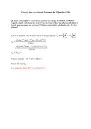
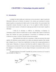
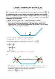
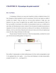
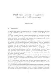
90 CHAPTER 5: Estimat<strong>in</strong>g <strong>of</strong> <strong>the</strong> <strong>Jet</strong> <strong>Energy</strong> <strong>Scale</strong> Calibration Factorfrom <strong>the</strong> decay <strong>of</strong> <strong>the</strong> top quark <strong>in</strong> <strong>the</strong> topology t → Wb → q¯qb. For a typical event,<strong>the</strong> distribution <strong>of</strong> <strong>the</strong> P K<strong>in</strong>Fit (∆E l , ∆E b ) is shown <strong>in</strong> Figure 5.12.P K<strong>in</strong>Fit(∆E l,∆E b)10.80.60.40.21.4 01.31.21.1∆E b10.90.80.70.60.6∆E l0.7 0.8 0.9 1 1.1 1.21.3 1.4Figure 5.12: The distribution <strong>of</strong> <strong>the</strong> P K<strong>in</strong>Fit (∆E l , ∆E b ) for an e+jets t¯t event.The central po<strong>in</strong>t <strong>of</strong> <strong>the</strong> distribution <strong>of</strong> <strong>the</strong> P K<strong>in</strong>Fit (∆E l , ∆E b ), which is expressedby P K<strong>in</strong>Fit (∆E l = 1, ∆E b = 1), corresponds to <strong>the</strong> situation when no correction isapplied. It is understood from Figure 5.12 that <strong>the</strong> maximum <strong>of</strong> <strong>the</strong> fit, for thatparticular event, does not happen at <strong>the</strong> center <strong>of</strong> <strong>the</strong> grid, which shows <strong>the</strong> need for<strong>the</strong> residual jet energy corrections. In order to justify <strong>the</strong> need for <strong>the</strong> residual jetenergy corrections, one has to <strong>in</strong>crease <strong>the</strong> statistics and may look at <strong>the</strong> distribution<strong>of</strong> <strong>the</strong> values <strong>of</strong> <strong>the</strong> P K<strong>in</strong>Fit (∆E l = 1, ∆E b = 1), which is shown <strong>in</strong> Figure 5.13.There is a clear peak at zero which can be partially <strong>in</strong>terpreted as follows. Thehypo<strong>the</strong>sis that <strong>the</strong> three jets <strong>in</strong> e+jets t¯t event orig<strong>in</strong>ate from <strong>the</strong> top quark is notfulfilled and <strong>the</strong> imposed mass constra<strong>in</strong>ts are not converged, when no correction isapplied. This observation justify <strong>the</strong> nead for <strong>the</strong> residual jet energy correction. Also<strong>the</strong> events, where <strong>the</strong> MVA method is not able to return <strong>the</strong> correct jet-parton comb<strong>in</strong>ation,contribute to <strong>the</strong> peak at zero as will be discussed <strong>in</strong> what follows.For a given event, <strong>the</strong> po<strong>in</strong>t with <strong>the</strong> maximum probability <strong>in</strong> <strong>the</strong> distribution <strong>of</strong> <strong>the</strong>P K<strong>in</strong>Fit (∆E l , ∆E b ), which is expressed by PK<strong>in</strong>Fit max (∆E l, ∆E b ), shows <strong>the</strong> po<strong>in</strong>t where<strong>the</strong> imposed constra<strong>in</strong>ts are maximally fulfilled. The distribution <strong>of</strong> <strong>the</strong> PK<strong>in</strong>Fit max (∆E l, ∆E b )value for all events that already pass <strong>the</strong> radiation veto cut, is shown <strong>in</strong> Figure 5.14.It is seen from Figure 5.14 that for most <strong>of</strong> <strong>the</strong> events, a maximum probabilityexceed<strong>in</strong>g 0.9 is returned by <strong>the</strong> k<strong>in</strong>ematic fit method, represent<strong>in</strong>g those events forwhich <strong>the</strong> maximum happens somewhere <strong>in</strong> <strong>the</strong> region that is scanned. Some <strong>of</strong> <strong>the</strong>events are peaked around zero which represent those events where no maximum is found<strong>in</strong> <strong>the</strong> w<strong>in</strong>dow <strong>of</strong> ±40% around <strong>the</strong> measured values <strong>of</strong> <strong>the</strong> jet energies or events that<strong>the</strong> fit is not converged for <strong>the</strong> given jet-parton comb<strong>in</strong>ation. This can be understoodby look<strong>in</strong>g at <strong>the</strong> two-dimensional histogram which is made by plott<strong>in</strong>g <strong>the</strong> distribution
CHAPTER 5: Estimat<strong>in</strong>g <strong>of</strong> <strong>the</strong> <strong>Jet</strong> <strong>Energy</strong> <strong>Scale</strong> Calibration Factor 91#Events210tt+jets semi-ele (180.4 entries)tt+jets o<strong>the</strong>r (22.5 entries)t+jets, (all channels) (9.9 entries)Z+jets (2.5 entries)W+jets (21.5 entries)Multi-jets (27.4 entries)10110-10 0.2 0.4 0.6 0.8 1K<strong>in</strong>Fit Probability without correctionsFigure 5.13: The distribution <strong>of</strong> <strong>the</strong> fit probability P K<strong>in</strong>Fit (∆E l = 1, ∆E b = 1) whenno correction is applied. All events surviv<strong>in</strong>g <strong>the</strong> radiation veto cut, are taken <strong>in</strong>toaccount.#Events21010tt+jets semi-ele (180.4 entries)tt+jets o<strong>the</strong>r (22.5 entries)t+jets, (all channels) (9.9 entries)Z+jets (2.5 entries)W+jets (21.5 entries)Multi-jets (27.4 entries)110-10 0.2 0.4 0.6 0.8 1max Probability <strong>of</strong> <strong>the</strong> K<strong>in</strong>FitFigure 5.14: The distribution <strong>of</strong> <strong>the</strong> maximum fit probability P maxK<strong>in</strong>Fit (∆E l, ∆E b ) among<strong>the</strong> fit values which are obta<strong>in</strong>ed <strong>in</strong> <strong>the</strong> scanned range around <strong>the</strong> uncorrected energies.All events survived <strong>the</strong> radiation veto cut, are taken <strong>in</strong>to account.