Arquivo do Trabalho - IAG - USP

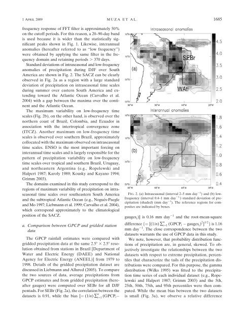
1APRIL 2009 M U Z A E T A L . 1685frequency response of FFT filter is approximately 50%on the cutoff periods. For this reason, a 20–90-day bandis used because it is wider than the statistically significantpeaks shown in Fig. 1. Likewise, interannualanomalies (hereafter referred to as ‘‘low frequency’’)were obtained by applying the same filter in the frequencydomain and retaining periods . 370 days.Standard deviations of intraseasonal and low-frequencyanomalies of precipitation during DJF over SouthAmerica are shown in Fig. 2. The SACZ can be clearlyobserved in Fig. 2a as a region with a large standarddeviation of precipitation on intraseasonal time scalesduring summer over eastern South America and extendingtoward the Atlantic Ocean (Carvalho et al.2004) with a gap between the maxima over the continentand the Atlantic Ocean.The maximum variability on low-frequency timescales (Fig. 2b), on the other hand, is observed over thenorthern coast of Brazil, Colombia, and Ecuador inassociation with the intertropical convergence zone(ITCZ). Another maximum on low-frequency timescales is observed over southern Brazil, approximatelycollocated with the maximum observed on intraseasonaltime scales. ENSO is the most important forcing oninterannual time scales and is largely responsible for thepattern of precipitation variability on low-frequencytime scales over tropical and southern Brazil, Uruguay,and northeastern Argentina (e.g., Ropelewski andHalpert 1987; Karoly 1989; Kousky and Kayano 1994;Grimm 2003).The domains examined in this study correspond to theregions of maximum variability of precipitation on intraseasonaltime scales over southeastern South Americaand the subtropical Atlantic Ocean (e.g., Nogués-Paegleand Mo 1997; Liebmann et al. 1999; Carvalho et al. 2004),which correspond approximately to the climatologicalposition of the SACZ.a. Comparison between GPCP and gridded stationdataThe GPCP rainfall estimates were compared withgridded precipitation data at the same 2.58 32.58 resolutionobtained from stations in Brazil [Department ofWater and Electric Energy (DAEE) and NationalAgency for Electric Energy (ANEEL)] from 1979 to1998. Details of the gridded precipitation dataset arediscussed in Liebmann and Allured (2005). To comparethe two sources of data, average precipitations fromGPCP estimates and from gridded precipitation (hereaftergauges) were computed over SEBr for all DJFpentads. For SEBr (Fig. 2a), the correlation between thedatasets is 0.91, while the bias [¼ (1/n) å n t¼1 (GPCP tFIG. 2. (a) Intraseasonal (interval 2–5 mm day 21 ) and (b) lowfrequency(interval 0.4–1 mm day 21, ) standard deviation of precipitation(shaded) (mm day 21 ). The reference regions for compositesare indicated by boxes.gauges t )] is 0.16 mm day 21 and the root-mean-squaredifference f¼ [(1/n) å n t¼1 (GPCP t gauges t ) 2 ] 1/2 g is 1.16mm day 21 . The close correspondence between the twodatasets warrants the use of GPCP data in this study.We note, however, that probability distribution functionsof precipitation are, in general, skewed. To objectivelyinvestigate the relationships between the twodatasets with respect to extreme precipitation, percentilesthat characterize the tails of the precipitation distributionswere compared. For this purpose, the gammadistribution (Wilks 1995) was fitted to the precipitationtime series of each individual dataset (e.g., Ropelewskiand Halpert 1987; Grimm 2003) and the 5th,25th, 50th, 75th, and 95th percentiles were then computed.While the mean bias between the two datasetsis small (Fig. 3a), we observe a relative difference