- Page 2:
This page intentionally left blank
- Page 6:
This is the first comprehensive tex
- Page 10:
cambridge university press Cambridg
- Page 14:
vi An Ode to the Unity of Time and
- Page 18:
viii Contents 4.5 Canonical quantiz
- Page 24:
Preface String theory is one of the
- Page 28:
Preface xiii stein of Caltech for t
- Page 32:
Preface xv NL, NR left- and right-m
- Page 36:
1 Introduction There were two major
- Page 40:
1.2 General features 3 theory fell
- Page 44:
1.2 General features 5 is only cons
- Page 48: 1.3 Basic string theory 7 world she
- Page 52: 1.4 Modern developments in superstr
- Page 56: 1.4 Modern developments in superstr
- Page 60: 1.4 Modern developments in superstr
- Page 64: 1.4 Modern developments in superstr
- Page 68: 2 The bosonic string This chapter i
- Page 72: 2.1 p-brane actions 19 choice of pa
- Page 76: particle, namely 2.1 p-brane action
- Page 80: SOLUTION 2.1 p-brane actions 23 The
- Page 84: where ˙X µ = ∂Xµ ∂τ 2.2 The
- Page 88: Tαβ, that is, 2.2 The string acti
- Page 92: 2.2 The string action 29 where we h
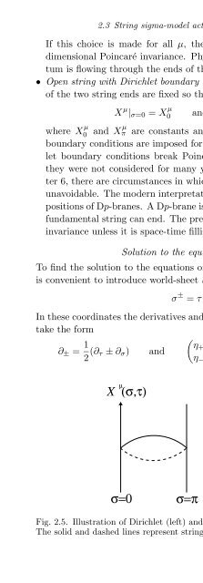
- Page 96: 2.3 String sigma-model action: the
- Page 102: 34 The bosonic string In light-cone
- Page 106: 36 The bosonic string 2.4 Canonical
- Page 110: 38 The bosonic string where φ is a
- Page 114: 40 The bosonic string where pµ is
- Page 118: 42 The bosonic string Using the com
- Page 122: 44 The bosonic string There are no
- Page 126: 46 The bosonic string Determination
- Page 130: 48 The bosonic string 2.5 Light-con
- Page 134: 50 The bosonic string Mass-shell co
- Page 138: 52 The bosonic string is made manif
- Page 142: 54 The bosonic string (i) Show that
- Page 146: 56 The bosonic string PROBLEM 2.6 E
- Page 150:
3 Conformal field theory and string
- Page 154:
60 Conformal field theory and strin
- Page 158:
62 Conformal field theory and strin
- Page 162:
64 Conformal field theory and strin
- Page 166:
66 Conformal field theory and strin
- Page 170:
68 Conformal field theory and strin
- Page 174:
70 Conformal field theory and strin
- Page 178:
72 Conformal field theory and strin
- Page 182:
74 Conformal field theory and strin
- Page 186:
76 Conformal field theory and strin
- Page 190:
78 Conformal field theory and strin
- Page 194:
80 Conformal field theory and strin
- Page 198:
82 Conformal field theory and strin
- Page 202:
84 Conformal field theory and strin
- Page 206:
86 Conformal field theory and strin
- Page 210:
88 Conformal field theory and strin
- Page 214:
90 Conformal field theory and strin
- Page 218:
92 Conformal field theory and strin
- Page 222:
94 Conformal field theory and strin
- Page 226:
96 Conformal field theory and strin
- Page 230:
98 Conformal field theory and strin
- Page 234:
100 Conformal field theory and stri
- Page 238:
102 Conformal field theory and stri
- Page 242:
104 Conformal field theory and stri
- Page 246:
106 Conformal field theory and stri
- Page 250:
108 Conformal field theory and stri
- Page 254:
110 Strings with world-sheet supers
- Page 258:
112 Strings with world-sheet supers
- Page 262:
114 Strings with world-sheet supers
- Page 266:
116 Strings with world-sheet supers
- Page 270:
118 Strings with world-sheet supers
- Page 274:
120 Strings with world-sheet supers
- Page 278:
122 Strings with world-sheet supers
- Page 282:
124 Strings with world-sheet supers
- Page 286:
126 Strings with world-sheet supers
- Page 290:
128 Strings with world-sheet supers
- Page 294:
130 Strings with world-sheet supers
- Page 298:
132 Strings with world-sheet supers
- Page 302:
134 Strings with world-sheet supers
- Page 306:
136 Strings with world-sheet supers
- Page 310:
138 Strings with world-sheet supers
- Page 314:
140 Strings with world-sheet supers
- Page 318:
142 Strings with world-sheet supers
- Page 322:
144 Strings with world-sheet supers
- Page 326:
146 Strings with world-sheet supers
- Page 330:
5 Strings with space-time supersymm
- Page 334:
150 Strings with space-time supersy
- Page 338:
152 Strings with space-time supersy
- Page 342:
154 Strings with space-time supersy
- Page 346:
156 Strings with space-time supersy
- Page 350:
158 Strings with space-time supersy
- Page 354:
160 Strings with space-time supersy
- Page 358:
162 Strings with space-time supersy
- Page 362:
164 Strings with space-time supersy
- Page 366:
166 Strings with space-time supersy
- Page 370:
168 Strings with space-time supersy
- Page 374:
170 Strings with space-time supersy
- Page 378:
172 Strings with space-time supersy
- Page 382:
174 Strings with space-time supersy
- Page 386:
176 Strings with space-time supersy
- Page 390:
178 Strings with space-time supersy
- Page 394:
180 Strings with space-time supersy
- Page 398:
182 Strings with space-time supersy
- Page 402:
184 Strings with space-time supersy
- Page 406:
186 Strings with space-time supersy
- Page 410:
188 T-duality and D-branes physical
- Page 414:
190 T-duality and D-branes where
- Page 418:
192 T-duality and D-branes Vα =
- Page 422:
194 T-duality and D-branes directio
- Page 426:
196 T-duality and D-branes Chan-Pat
- Page 430:
198 T-duality and D-branes mitian m
- Page 434:
200 T-duality and D-branes If two
- Page 438:
202 T-duality and D-branes X µ R =
- Page 442:
204 T-duality and D-branes space va
- Page 446:
206 T-duality and D-branes one-form
- Page 450:
208 T-duality and D-branes to a D3-
- Page 454:
210 T-duality and D-branes and Diri
- Page 458:
212 T-duality and D-branes where A
- Page 462:
214 T-duality and D-branes account
- Page 466:
216 T-duality and D-branes µp Ap+
- Page 470:
218 T-duality and D-branes EXERCISE
- Page 474:
220 T-duality and D-branes directio
- Page 478:
222 T-duality and D-branes Anomalie
- Page 482:
224 T-duality and D-branes the hete
- Page 486:
226 T-duality and D-branes gauge sy
- Page 490:
228 T-duality and D-branes D-branes
- Page 494:
230 T-duality and D-branes spinors,
- Page 498:
232 T-duality and D-branes By T-dua
- Page 502:
234 T-duality and D-branes One reas
- Page 506:
236 T-duality and D-branes and in t
- Page 510:
238 T-duality and D-branes the Cher
- Page 514:
240 T-duality and D-branes which ar
- Page 518:
242 T-duality and D-branes matrix,
- Page 522:
244 T-duality and D-branes What typ
- Page 526:
246 T-duality and D-branes PROBLEM
- Page 530:
248 T-duality and D-branes PROBLEM
- Page 534:
250 The heterotic string string the
- Page 538:
252 The heterotic string 7.2 Fermio
- Page 542:
254 The heterotic string where µ =
- Page 546:
256 The heterotic string Left-mover
- Page 550:
258 The heterotic string which is a
- Page 554:
260 The heterotic string it is natu
- Page 558:
262 The heterotic string even, and
- Page 562:
264 The heterotic string where λ A
- Page 566:
266 The heterotic string The bosoni
- Page 570:
268 The heterotic string KI, which
- Page 574:
270 The heterotic string following.
- Page 578:
272 The heterotic string • The Fo
- Page 582:
274 The heterotic string In the cas
- Page 586:
276 The heterotic string Modular in
- Page 590:
278 The heterotic string The metric
- Page 594:
280 The heterotic string the circle
- Page 598:
282 The heterotic string as require
- Page 602:
284 The heterotic string contributi
- Page 606:
286 The heterotic string symmetry.
- Page 610:
288 The heterotic string Duality an
- Page 614:
290 The heterotic string (ii) (iii)
- Page 618:
292 The heterotic string SO(32) cur
- Page 622:
294 The heterotic string whose inne
- Page 626:
8 M-theory and string duality Durin
- Page 630:
298 M-theory and string duality bel
- Page 634:
300 M-theory and string duality cha
- Page 638:
302 M-theory and string duality Ele
- Page 642:
304 M-theory and string duality are
- Page 646:
306 M-theory and string duality The
- Page 650:
308 M-theory and string duality in
- Page 654:
310 M-theory and string duality tra
- Page 658:
312 M-theory and string duality Eq.
- Page 662:
314 M-theory and string duality The
- Page 666:
316 M-theory and string duality tra
- Page 670:
318 M-theory and string duality Res
- Page 674:
320 M-theory and string duality giv
- Page 678:
322 M-theory and string duality SOL
- Page 682:
324 M-theory and string duality sup
- Page 686:
326 M-theory and string duality wha
- Page 690:
328 M-theory and string duality are
- Page 694:
330 M-theory and string duality dua
- Page 698:
332 M-theory and string duality M-b
- Page 702:
334 M-theory and string duality Sin
- Page 706:
336 M-theory and string duality ten
- Page 710:
338 M-theory and string duality het
- Page 714:
340 M-theory and string duality and
- Page 718:
342 M-theory and string duality Thu
- Page 722:
344 M-theory and string duality dim
- Page 726:
346 M-theory and string duality cas
- Page 730:
348 M-theory and string duality Wha
- Page 734:
350 M-theory and string duality ten
- Page 738:
352 M-theory and string duality PRO
- Page 742:
9 String geometry Since critical su
- Page 746:
356 String geometry At sufficiently
- Page 750:
358 String geometry Fig. 9.1. This
- Page 754:
360 String geometry Noncompact exam
- Page 758:
362 String geometry In the quantum
- Page 762:
364 String geometry of the manifold
- Page 766:
366 String geometry 9.3 Examples of
- Page 770:
368 String geometry Hodge numbers o
- Page 774:
370 String geometry is a compact K
- Page 778:
372 String geometry proportional to
- Page 782:
374 String geometry This leads to t
- Page 786:
376 String geometry independent cho
- Page 790:
378 String geometry This implies th
- Page 794:
380 String geometry Kähler form an
- Page 798:
382 String geometry satisfies √ g
- Page 802:
384 String geometry In writing this
- Page 806:
386 String geometry This section an
- Page 810:
388 String geometry torus is descri
- Page 814:
390 String geometry where Mr is any
- Page 818:
392 String geometry Writing the met
- Page 822:
394 String geometry Since the prepo
- Page 826:
396 String geometry A change in the
- Page 830:
398 String geometry For these choic
- Page 834:
400 String geometry coefficients. W
- Page 838:
402 String geometry four fermionic
- Page 842:
404 String geometry a vanishing cyc
- Page 846:
406 String geometry global supersym
- Page 850:
408 String geometry similar fashion
- Page 854:
410 String geometry where K = 1 2 (
- Page 858:
412 String geometry versa. An early
- Page 862:
414 String geometry by complex-stru
- Page 866:
416 String geometry holonomy group,
- Page 870:
418 String geometry rather than SU(
- Page 874:
420 String geometry to the case of
- Page 878:
422 String geometry For example, in
- Page 882:
424 String geometry example is the
- Page 886:
426 String geometry type IIA string
- Page 890:
428 String geometry which transform
- Page 894:
430 String geometry The tension of
- Page 898:
432 String geometry fibration. Only
- Page 902:
434 String geometry folds, constrai
- Page 906:
436 String geometry to that in Exer
- Page 910:
438 String geometry be interpreted
- Page 914:
440 String geometry SOLUTION An inf
- Page 918:
442 String geometry to a zero form
- Page 922:
444 String geometry Riemannian geom
- Page 926:
446 String geometry map tensors to
- Page 930:
448 String geometry a possible holo
- Page 934:
450 String geometry as the complex
- Page 938:
452 String geometry . ✷ EXERCISE
- Page 942:
454 String geometry PROBLEM 9.8 Use
- Page 946:
10 Flux compactifications Moduli-sp
- Page 950:
458 Flux compactifications This hap
- Page 954:
460 Flux compactifications the stan
- Page 958:
462 Flux compactifications coordina
- Page 962:
464 Flux compactifications Fig. 10.
- Page 966:
466 Flux compactifications The last
- Page 970:
468 Flux compactifications forms (a
- Page 974:
470 Flux compactifications G µν G
- Page 978:
472 Flux compactifications Fig. 10.
- Page 982:
474 Flux compactifications Superpot
- Page 986:
476 Flux compactifications where dz
- Page 990:
478 Flux compactifications Since m
- Page 994:
480 Flux compactifications 10.2 Flu
- Page 998:
482 Flux compactifications is the e
- Page 1002:
484 Flux compactifications the fibe
- Page 1006:
486 Flux compactifications The tota
- Page 1010:
488 Flux compactifications S 3 S 2
- Page 1014:
490 Flux compactifications be true
- Page 1018:
492 Flux compactifications where gs
- Page 1022:
494 Flux compactifications Fig. 10.
- Page 1026:
496 Flux compactifications Negative
- Page 1030:
498 Flux compactifications will be
- Page 1034:
500 Flux compactifications As you a
- Page 1038:
502 Flux compactifications where K
- Page 1042:
504 Flux compactifications is of in
- Page 1046:
506 Flux compactifications V(σ) Fi
- Page 1050:
508 Flux compactifications where Da
- Page 1054:
510 Flux compactifications Fig. 10.
- Page 1058:
512 Flux compactifications M, N, P
- Page 1062:
514 Flux compactifications By defin
- Page 1066:
516 Flux compactifications In this
- Page 1070:
518 Flux compactifications As a res
- Page 1074:
520 Flux compactifications constant
- Page 1078:
522 Flux compactifications a way th
- Page 1082:
524 Flux compactifications F3 −
- Page 1086:
526 Flux compactifications One fina
- Page 1090:
528 Flux compactifications Friedman
- Page 1094:
530 Flux compactifications If there
- Page 1098:
532 Flux compactifications cosmolog
- Page 1102:
534 Flux compactifications to Eq. (
- Page 1106:
536 Flux compactifications but not
- Page 1110:
538 Flux compactifications e-foldin
- Page 1114:
540 Flux compactifications of makin
- Page 1118:
542 Flux compactifications Here W0
- Page 1122:
544 Flux compactifications [γmn,
- Page 1126:
546 Flux compactifications complex
- Page 1130:
548 Flux compactifications Eq. (10.
- Page 1134:
550 Black holes in string theory th
- Page 1138:
552 Black holes in string theory di
- Page 1142:
554 Black holes in string theory He
- Page 1146:
556 Black holes in string theory r=
- Page 1150:
558 Black holes in string theory
- Page 1154:
560 Black holes in string theory of
- Page 1158:
562 Black holes in string theory Th
- Page 1162:
564 Black holes in string theory wh
- Page 1166:
566 Black holes in string theory SO
- Page 1170:
568 Black holes in string theory Th
- Page 1174:
570 Black holes in string theory st
- Page 1178:
572 Black holes in string theory M-
- Page 1182:
574 Black holes in string theory ro
- Page 1186:
576 Black holes in string theory In
- Page 1190:
578 Black holes in string theory Fi
- Page 1194:
580 Black holes in string theory (2
- Page 1198:
582 Black holes in string theory SO
- Page 1202:
584 Black holes in string theory ju
- Page 1206:
586 Black holes in string theory No
- Page 1210:
588 Black holes in string theory co
- Page 1214:
590 Black holes in string theory ba
- Page 1218:
592 Black holes in string theory Th
- Page 1222:
594 Black holes in string theory Fi
- Page 1226:
596 Black holes in string theory su
- Page 1230:
598 Black holes in string theory wh
- Page 1234:
600 Black holes in string theory 28
- Page 1238:
602 Black holes in string theory is
- Page 1242:
604 Black holes in string theory wh
- Page 1246:
606 Black holes in string theory S-
- Page 1250:
608 Black holes in string theory PR
- Page 1254:
12 Gauge theory/string theory duali
- Page 1258:
612 Gauge theory/string theory dual
- Page 1262:
614 Gauge theory/string theory dual
- Page 1266:
616 Gauge theory/string theory dual
- Page 1270:
618 Gauge theory/string theory dual
- Page 1274:
620 Gauge theory/string theory dual
- Page 1278:
622 Gauge theory/string theory dual
- Page 1282:
624 Gauge theory/string theory dual
- Page 1286:
626 Gauge theory/string theory dual
- Page 1290:
628 Gauge theory/string theory dual
- Page 1294:
630 Gauge theory/string theory dual
- Page 1298:
632 Gauge theory/string theory dual
- Page 1302:
634 Gauge theory/string theory dual
- Page 1306:
636 Gauge theory/string theory dual
- Page 1310:
638 Gauge theory/string theory dual
- Page 1314:
640 Gauge theory/string theory dual
- Page 1318:
642 Gauge theory/string theory dual
- Page 1322:
644 Gauge theory/string theory dual
- Page 1326:
646 Gauge theory/string theory dual
- Page 1330:
648 Gauge theory/string theory dual
- Page 1334:
650 Gauge theory/string theory dual
- Page 1338:
652 Gauge theory/string theory dual
- Page 1342:
654 Gauge theory/string theory dual
- Page 1346:
656 Gauge theory/string theory dual
- Page 1350:
658 Gauge theory/string theory dual
- Page 1354:
660 Gauge theory/string theory dual
- Page 1358:
662 Gauge theory/string theory dual
- Page 1362:
664 Gauge theory/string theory dual
- Page 1366:
666 Gauge theory/string theory dual
- Page 1370:
668 Gauge theory/string theory dual
- Page 1374:
670 Gauge theory/string theory dual
- Page 1378:
672 Gauge theory/string theory dual
- Page 1382:
674 Gauge theory/string theory dual
- Page 1386:
676 Gauge theory/string theory dual
- Page 1390:
678 Gauge theory/string theory dual
- Page 1394:
680 Gauge theory/string theory dual
- Page 1398:
682 Gauge theory/string theory dual
- Page 1402:
684 Gauge theory/string theory dual
- Page 1406:
686 Gauge theory/string theory dual
- Page 1410:
688 Gauge theory/string theory dual
- Page 1414:
Bibliographic discussion In the fol
- Page 1418:
692 Bibliographic discussion The BR
- Page 1422:
694 Bibliographic discussion derive
- Page 1426:
696 Bibliographic discussion which
- Page 1430:
698 Bibliographic discussion Maldac
- Page 1434:
Bibliography Abouelsaood, A., Calla
- Page 1438:
702 Bibliography Singapore: World S
- Page 1442:
704 Bibliography Brink, L., and Nie
- Page 1446:
706 Bibliography E-print hep-th/000
- Page 1450:
708 Bibliography hep-th/0105203. Eg
- Page 1454:
710 Bibliography Phys., 71, 983-108
- Page 1458:
712 Bibliography hep-th/9802109. Gu
- Page 1462:
714 Bibliography Johnson, C. V. (20
- Page 1466:
716 Bibliography Lerche, W., Schell
- Page 1470:
718 Bibliography Montonen, C. (1974
- Page 1474:
720 Bibliography Polchinski, J., an
- Page 1478:
722 Bibliography Sen, A. (1999). No
- Page 1482:
724 Bibliography Tseytlin, A. A. (1
- Page 1486:
acceleration equation, 528 action p
- Page 1490:
728 Index Calabi-Yau four-fold, 458
- Page 1494:
730 Index with E6,6 symmetry, 570 c
- Page 1498:
732 Index Friedmann equation, 528 F
- Page 1502:
734 Index dual Coxeter number, 69 e
- Page 1506:
736 Index homogeneity equation, 603
- Page 1510:
738 Index superconformal symmetry,