European Journal of Scientific Research - EuroJournals

Model-Based Adaptive Chaos Control using Lyapunov Exponents 327
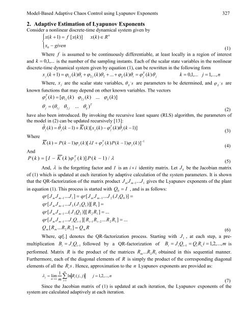
2. Adaptive Estimation of Lyapunov Exponents
Consider a nonlinear discrete-time dynamical system given by
n
⎪⎧
x(
k + 1)
= f [ x(
k)]
x(
k)
∈ R
⎨
⎪⎩ x0
− given
(1)
Where f is assumed to be continuously differentiable, at least locally in a region of interest
and k = 0,
1,...
is the number of the sampling instants. Each of the scalar state variables in the nonlinear
discrete-time dynamical system given by equation (1), can be rewritten in the following form
T
x j ( k + 1)
= ϕ 1 j ( k)
θ1
+ ϕ2
j ( k)
θ 2 + ... + ϕij
( k)
θi
= ϕ j ( k)
θ j k = 0,
1,...
j = 1,...,
n
,
,
Where, x j are the scalar state variables, θ ij s are parameters to be determined, and ϕ ij s are
known functions that may depend on other known variables. The vectors
T
ϕ ( k)
= [ ϕ ( k)
ϕ ( k)
... ϕ ( k)]
j
1 j
2 j
ij
θ j = ( θ1
j θ2
j ...
T
θij
)
(2)
have also been introduced. By invoking the recursive least square (RLS) algorithm, the parameters of
the model in (2) can be updated recursively [13]:
ˆ ˆ
T
θ ( ) ( 1)
( )[ ( ) ( ) ˆ
j k = θ j k − + K k x j k −ϕ
j k θ j ( k −1)]
(3)
Where
T
−1
K ( k ) = P(
k −1)
ϕ j ( k )[ λI
+ ϕ j ( k ) P(
k −1)
ϕ j ( k )]
(4)
And
T
P ( k ) = [ I − K ( k ) ϕ j ( k )] P ( k − 1)
/ λ
(5)
And, λ is the forgetting factor and I is an i × i identity matrix. Let J k be the Jacobian matrix
of (1) which is updated at each iteration by adaptive calculation of the system parameters. It is shown
that the QR-factorization of the matrix product J m J m−
1...J1
gives the Lyapunov exponents of the plant
in equation (1). This process is started with Q 0 = I , and is as follows:
qr[
J J ... J ] = qr[
J J ... J ( J Q )] =
qr[
J
qr[
J
qr[
J
m
m
m
m
J
J
J
m−1
m−1
m−1
m−1
... J
...( J Q )][ R R ] = ...
... J
1
3
i
( J Q )][ R ] =
3
Q
2
2
i−1
1
][ R
m
2
i−1
R
m−1
1
1
i−
2
... R
2
2
R
1
1
0
] = ...
Qm
[ Rm
... R2
R1]
= Qm
R
(6)
Where, qr[.] denotes the QR-factorization process. Starting with J 1 , at each step, a pre-
B J Q followed by a QR-factorization of = J Q − = Q R i = 1,
2,...,
m is
multiplication i = i i−1
performed. Matrix R is the product of the matrices ... R2R1
Bi i i 1 i i,
Rm obtained in this sequential manner.
Furthermore, each of the diagonal elements of R is simply the product of the corresponding diagonal
elements of all the
,
s . Hence, approximation to the n Lyapunov exponents are provided as:
R i
m 1
λ j = lim ∑ ln Ri
( j,
j)
j = 1,
2,...,
n
m→∞
m i=
1
(7)
Since the Jacobian matrix of (1) is updated at each iteration, the Lyapunov exponents of the
system are calculated adaptively at each iteration.