Tutorial: EMC & Signal Integrity using SPICE, page 44 - IEEE EMC ...
Tutorial: EMC & Signal Integrity using SPICE, page 44 - IEEE EMC ...
Tutorial: EMC & Signal Integrity using SPICE, page 44 - IEEE EMC ...

You also want an ePaper? Increase the reach of your titles
YUMPU automatically turns print PDFs into web optimized ePapers that Google loves.
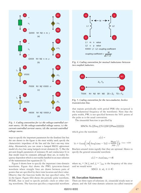
i x<br />
i x<br />
+<br />
–<br />
+ –<br />
n<br />
m<br />
n<br />
m<br />
n<br />
m<br />
+<br />
v x<br />
–<br />
GXXX<br />
N1 N2 n m γ<br />
(a)<br />
ways to specify the important parameters for the (lossless) line but<br />
the one shown in the figure is the most widely used; specify the<br />
characteristic impedance of the line and the line’s one-way time<br />
delay. Alternatively you can create a lumped RLCG approximate<br />
model of a lossy line <strong>using</strong> lumped-circuit elements [6, 7]. But the<br />
per-unit-length parameters of resistance R and conductance G in<br />
that model must be constants although these are, in reality frequency<br />
dependent which is not readily handled in an exact solution<br />
of the transmission-line equations [6–7].<br />
Figure 6 shows how to specify the important time-domain<br />
waveforms. Figure 6(a) shows the PWL (piecewise-linear)<br />
waveform where straight lines are drawn between pairs of<br />
points that are specified by their time location and their value.<br />
Observe that the function holds the last specified value, V4<br />
in the figure. Figure 6(b) shows the periodic pulse waveform,<br />
PULSE, that is used to specify periodic clock or other timing<br />
waveforms. The function specifies a trapezoidal waveform<br />
� v x<br />
VXXX � i x<br />
n<br />
+<br />
v x<br />
–<br />
VXXX<br />
m<br />
EXXX<br />
FXXX<br />
HXXX<br />
N1 N2 n m α<br />
(b)<br />
N1 N2 VXXX σ<br />
(c)<br />
N1 N2 VXXX β<br />
(d)<br />
+<br />
–<br />
� v x<br />
Fig. 3. Coding convention for (a) the voltage-controlled current<br />
source, (b) the voltage-controlled voltage source, (c) the<br />
current-controlled current source, (d) the current-controlled<br />
voltage source.<br />
+ –<br />
N1<br />
N2<br />
N1<br />
N2<br />
N1<br />
N2<br />
N1<br />
� i x<br />
N2<br />
©2010 <strong>IEEE</strong><br />
m<br />
that repeats periodically with period PER (the reciprocal is<br />
the fundamental frequency of the waveform). Note that the<br />
pulse width, PW, is not specified between the 50% points of<br />
the pulse as is the usual convention.<br />
The sinusoidal function is specified by<br />
SIN(Vo Va [[Freq [[Td [[Df [[Phase]]]]]]]])<br />
which gives the waveform<br />
n<br />
L1<br />
L2<br />
M<br />
L1 L2<br />
m<br />
o<br />
n value<br />
p<br />
value<br />
KXXX L1 L2 coupling coefficient<br />
coupling coefficient =<br />
x1t2 5<br />
L1 L2<br />
Fig. 4. Coding convention for mutual inductance between<br />
two coupled inductors.<br />
N1<br />
N2<br />
TXXX<br />
N1<br />
N2<br />
Z C , T D<br />
M1<br />
M2<br />
Vo 1 Vasina2paFreq1time 2 Td2 1 Phase<br />
b be21time2Td2Df<br />
360<br />
Brackets around items signify that they are optional. Hence to<br />
specify the general sinusoidal waveform<br />
x1t2 5 Asin1nv 0t 1 u2<br />
where v 0 5 2p f 0 and f 0 5 1 @PER is the frequency of the sinusoid<br />
we would write<br />
SIN10 A nf 0 0 0 u 2<br />
iii. execution Statements<br />
There are three types of solutions: dc, sinusoidal steady state or<br />
phasor, and the full time-domain solution (so-called transient<br />
M<br />
Z0 = Z C<br />
o<br />
p<br />
M1<br />
M2<br />
TD = T D<br />
Fig. 5. Coding convention for the two-conductor, lossless<br />
transmission line.<br />
47