Tutorial: EMC & Signal Integrity using SPICE, page 44 - IEEE EMC ...

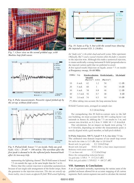
Fig. 7. Closer view on the second gridded cage, with
Moebius loop field sensor.
TeK Arret
^
1
T
Ch1 1.00 mVΩ M 20.0ns
Fig. 8. Pulse measurements. Parasitic signal picked-up by
the set-up, without field sensor.
TeK Arret
^
1
T
T 20.00 %
Ch1 20.0 mVΩ M 10.0ns
T
T
T 14.00 %
A Ch1 720µV
A Ch1 –74.8mV
∆: 280µV
@: 60.0µV
∆: 12.8ns
@: –126ns
7 Sep 2005
09:38:36
∆: 47.2mV
@: –800µV
∆: 12.8ns
@: –5.60ns
7 Sep 2005
09:47:40
Fig. 9. Pulsed field. Sensor 7.5 cm inside. Only one grid.
Scale : Ch.1 : 20 mV 5 100 mA/m. The overshoot after the
first peak is deemed to be the reflected pulse bounced-back
after its two-way trip.
representing the lightning channel. The H-field sensor is located
7.5 cm outside the cage, at the same height than for 5 or 6).
Notice that this current injection is somewhat asymmetrical,
because of our single-side arrangement of the feeder stripe, from
the generator to the injection structure. This does not correctly replicates
reality, since it creates an opposite H-field. With actual lightning,
64 ©2010 IEEE
2
TeK Arret
^
T
T
Ch1 50.0mVΩ Ch2 2.00 A M 20.0ns Ch1 –75.0mV
T 14.00 %
Fig. 10. Same as Fig. 9, but with the second trace showing
the injected current (Ch. 2: 2A/div).
the “feeder wire” is the whole cloud -and-earth system. Other experiments
(Metwally, Ref.7) used a coaxial structure where the feeder is concentric
to the injection wire. Although this make a symetrical injection,
it creates artificially a strong horizontal E-field (perpendicular to
the injected current path) that we preferred to avoid.
A few typical results (Injection on façade, sensor 7.5 cm inside)
a) Frequency sweep, 10–60 MHz
F(MHz) I inj. H in the x direction, H with 2nd grid S.E, 2nd grid
(one grid)
dBµA/m(*) mA/m dBµA/m(*)
10 6 mA 62 1.2 50 12 dB
20 5 mA 60 1 50 10 dB
30 4 mA 58 0.8 46 12 dB
40 3.5 mA 56 0.7 48 8 dB
50 2.6 mA 54 0.5 44 10 dB
(*) After taking into account the loop antenna factor.
H-field/ Current ratio, averaged on sample size:
0.2 (A/m)/Amp
∆: 9.56 A
@: –9.72 A
Ch1 Ampl
141.5mV
7 Sep 2005
09:57:33
For extrapolating this H field-to-current ratio to the full
size building, we must account for the 40/1 scaling factor ( see
rationale in Annex A), shifting the 7.5 cm results to 3 m, and
convert into A/m/kA, so: 0.2 A/m 3 1000/ 40 5 (5 A/m)/kA
Our calculations, for an impact on façade were giving 7.6
to 9 A/m/kA, depending on wether the measurement point is
exactly aligned with a grid member, or half-pitch shifted.
b) Pulse Injection, 500 V, I peak 5 8 A, rise time 7.5 ns.
The calibrated time-domain response of our small loop sensor
for such rise time is 13.5 dB, that is 4.8 A/m/V
Result with 1st grid only: 0.1 1A/m2 /Amp
Result with 2nd grid: 0.022 A/m ( a four times improvement)
Reference with sensor outside, at
7.5 cm from rod: 1.5 1A/m2 /Amp
Hence the corresponding reduction factors:
1st grid only: 1.5/0.1 5 15 123.5 dB2
With 2nd grid added: 1.5/0.022 5 68 137 dB2
Viii. Summary & conclusions
A set of equivalent networks, representing the various zones of the
gridded enclosure allowed for an accurate mapping of all current
segments. Each current segment was used to calculate the internal
A