Tutorial: EMC & Signal Integrity using SPICE, page 44 - IEEE EMC ...
Tutorial: EMC & Signal Integrity using SPICE, page 44 - IEEE EMC ...
Tutorial: EMC & Signal Integrity using SPICE, page 44 - IEEE EMC ...

Create successful ePaper yourself
Turn your PDF publications into a flip-book with our unique Google optimized e-Paper software.
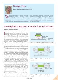
V 3<br />
V 4<br />
V 1<br />
V 2<br />
V 2<br />
V 1<br />
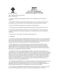
t1 t2 t3 t4 PWL (0 0 t1 V1 t2 V2 t3 V3 t4 V4 )<br />
TD TR PW TF PER<br />
Pulse (V1 V2 TD TR TF PW PER)<br />
(b)<br />
although it contains both the transient and the steady-state<br />
parts of the solution).<br />
The dc solution is specified by<br />
.DC V,IXXX start_value end_value increment<br />
where V,IXXX is the name of a dc voltage or current source in<br />
the circuit whose value is to swept. For example to sweep the<br />
value of a dc voltage source VFRED from 1 V to 10 V in increments<br />
of 2 V and solve the circuit for each of these source values<br />
we would write<br />
.DC VFRED 1 10 2<br />
If no sweeping of any source is desired then simply choose one dc<br />
source in the circuit and iterate its value from the actual value to<br />
the actual value and use any nonzero increment. For example,<br />
.DC VFRED 5 5 1<br />
The sinusoidal steady-state or phasor solution is specified by<br />
(a)<br />
.AC {LIN,DEC,OCT} points start_ frequency end_ frequency<br />
LIN denotes a linear frequency sweep from start_ frequency to<br />
end_ frequency and points is the total number of frequency<br />
points. DEC denotes a log sweep of the frequency where the<br />
frequency is swept logarithmically from the start_ frequency<br />
48 ©2010 <strong>IEEE</strong><br />
time<br />
time<br />
Fig. 6. Coding convention for the important source waveforms:<br />
(a) the piecewise-linear waveform and (b) the pulse<br />
source waveform (periodic).<br />
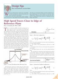
500 Ω<br />
5 V<br />
500<br />
5<br />
2<br />
+<br />
–<br />
+<br />
–<br />
1<br />
1 kΩ<br />
1000<br />
2 kΩ<br />
500i x<br />
500 Ω<br />
to the end_ frequency and points is the number of frequency<br />
points per decade. OCT is a log sweep by octaves where<br />
points is the number of frequency points per octave.<br />
The time-domain solution is obtained by specifying<br />
.TRAN print_step end_time [no_ print_time] [step_ceiling] [UIC]<br />
<strong>SPICE</strong> solves the time-domain differential equations of the<br />
circuit by discretizing the time variable into increments of<br />
Dt and solving the equations in a boot-strapping manner.<br />
The differential equations of the circuit are first solved at<br />
t 5 0 Then that solution is used to give the solution at t 5 Dt.<br />
These prior time solutions are then used to give the solution<br />
at t 5 2Dt and so on. The first item, print_step, governs when<br />
an output is requested. Suppose the discretization used in the<br />
solution is every 2ms. We might not want to see (in the output<br />
generated by the .PRINT statement) an output at every<br />
2ms but only every 5ms. Hence we might set the print_step<br />
time as 5M. The end_time is the final time that the solution<br />
is obtained for. The remaining parameters are optional. The<br />
analysis always starts at t 5 0. But we may not wish to see a<br />
printout of the solution (in the output generated by the<br />
.PRINT statement) until after some time has elapsed. If so<br />
we would set the no_ print_time to that starting time. <strong>SPICE</strong><br />
and Pspice have a very sophisticated algorithm for determining<br />
the minimum step size, Dt, for discretization of the differential<br />
equations in order to get a valid solution. The<br />
default maximum step size is end_time/50. However, there are<br />
many cases where we want the step size to be smaller than<br />
what <strong>SPICE</strong> would allow in order to increase the accuracy of<br />
the solution or to increase the resolution of the solution<br />
waveforms. This is frequently the case when we use <strong>SPICE</strong> in<br />
the analysis of transmission lines where abrupt waveform<br />
transitions are occurring at every one-way time delay. The<br />
step_ceiling is the maximum time step size, Dt 0 max, that will<br />
be used in discretizing the differential equations as described<br />
i x<br />
B<br />
4<br />
3<br />
+ –<br />
0<br />
i x<br />
+ –<br />
+<br />
V out<br />
–<br />
500i x<br />
+ –<br />
2000<br />
i<br />
5<br />
500<br />
6<br />
+ – 0<br />
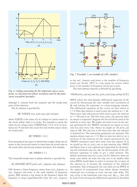
Fig. 7. Example 1, an example of a DC analysis.<br />
0<br />
i