Tutorial: EMC & Signal Integrity using SPICE, page 44 - IEEE EMC ...

2 2
2
Htot 5 U Hx1 Hy 1 Hz So, the amplitude of this ultimate vector H tot is always
greater than the largest of its components, giving the worst
possible exposure for the illuminated victim cable loops and
equipments inside.
Results are shown in A/m for 1 kA injected in Fig. 4. From
this, H can be extrapolated for any value of lightning current.
For visibility, some true values of H have been also displayed for
the 200 kA/10 ms and 50 kA/0.25 ms strokes.
Calculated values of E field are comparatively higher for the
subsequent stroke than for the “slow” one, because of the front
steepness (0.25 ms) forcing a higher wave impedance.
B. Example of Lightning Current
Distribution in a Corner Zone
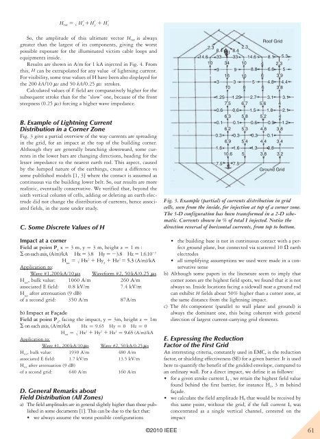
Fig. 3 give a partial overview of the way currents are spreading
in the grid, for an impact at the top of the building corner.
Although they are generally branching downward, some currents
in the lower bars are changing directions, heading for the
lesser impedance to the nearest earth rod. This aspect, caused
by the lumped nature of the earthings, create a difference vs
some published models [1, 3] where the contact is assumed as
continuous via the building lower belt. So, our results are more
realistic, eventually conservative. We verified that, beyond the
sixth vertical column of cells, adding or deleting an earth electrode
did not change the distribution of currents, hence associated
fields, in the zone under study.
C. Some Discrete Values of H
impact at a corner
Field at point P 1 x 5 3 m, y 5 3 m, height z 5 1 m :
S on each axis, (A/m)/kA Hx 5 3.8 Hy 5 23.8 Hz 5 1.6.10 23
H tot 5 U Hx 2 1 Hy 2 1 Hz 2 5 5.3 (A/m)/kA
Application to:
Wave #1,200 kA/10 ms Waveform #2, 50 kA/0.25 ms
H tot , bulk value: 1060 A/m 260 A/m
associated E field: 0.8 kV/m 7.4 kV/m
H tot after attenuation (9 dB)
of a second grid: 350 A/m 87A/m
b) Impact at Façade
Field at point P 2 , facing the impact, y 5 3m, height z 5 1m
S on each axis, (A/m)/kA Hx 5 9.65 Hy 5 0 Hz 5 0
H tot 5 U Hx 2 1 Hy 2 1 Hz 2 5 9.65 (A/m)/kA
Application to:
Wave #1, 200 kA/10 ms Wave #2, 50 kA/0.25 ms
H tot, bulk value: 1930 A/m 480 A/m
associated E field: 1.7 kV/m 13.5 kV/m
H tot after attenuation (9 dB)
of a second grid: 640 A/m 160 A/m
D. General Remarks about
Field Distribution (All Zones)
a) The field amplitudes are in general slightly higher than those published
in some documents [1]. This can be due to the fact that:
• we always assume the worst possible configurations
©2010 IEEE
Roof Grid
2.3
8.4
14.6 33
I
2.3
8.4
33 14.6
8.1 5.3
10 34 10 4 2.3
9 9 8.8 6.6 5
16 10 6 3.9
3 3 5 4.8 4.4
10 8 6 3.8
1.25 1.25 2.7 3.1 3.1
7.5 6.7 5.6 4
0.6 0.6 1.5 1.8 2.1
6.3 5.8 5.2 4
0.1 0.1 0.6 0.9 1.2
6.2 5.3 4.8 3.8
0.3 0.3 0.3 0.1
6.9 5.4 4.4 3.4
1.6 1.6 1.3 0.8
10.6 5 3.8 3.2
7.5 7.5
Ground Grid
Fig. 3. Example (partial) of currents distribution in grid
cells, seen from the inside, for injection at top of a corner zone.
The 3-D configuration has been transformed in a 2-D schematic.
Currents shown in % of total I injected. Notice the
direction reversal of horizontal currents, from top to bottom.
• the building base is not in continuous contact with a perfect
ground plane, but connected via scattered 10 V earth
electrodes
• all simplifying assumptions we used were made in a conservative
sense
b) Although some papers in the literature seem to imply that
corner zones are the highest field spots, we found that it is not
always so. Inside locations facing a sidewall near a ground rod
can exhibit H fields about 50% higher than a corner zone, at
the same distance from the lightning impact.
c) The Hx component (parallel to wall plane and ground) is
always the dominant one, this being coherent with general
direction of largest current-carrying grid elements.
E. Expressing the Reduction
Factor of the First Grid
An interesting criteria, constantly used in EMC, is the reduction
factor, or shielding effectiveness (SE) for a given barrier. It is used
here to quantify the benefit of the gridded envelope, compared to
an ordinary wall. For a direct impact, we define it as follows:
• for a given stroke current I0
, we retain the highest field value
found behind the first barrier, for instance Hx, 3 m behind
façade.
• we calculate the field amplitude H0
that would be received by
this same point, without the grid, if the full current I0 was
concentrated as a single vertical channel, centered on the
impact
61