cahier scientifique revue technique luxembourgeoise

Flux flange-slab (kW/m²)
40
35
30
25
20
15
10
5
42 CAHIER SCIENTIFIQUE | REVUE TECHNIQUE LUXEMBOURGEOISE 2 | 2010
�
�
heating
discontinuities observed around 735°C are due to the peak
value of the specifi c heat of steel at this temperature.
�
�
heating
heating
�T� �T � 20�
�150 � 20�
� �
; T � 150�C
(Eq. 9a)
(Eq. 9b)
(Eq. 9c)
(Eq. 9d)
� = 0.4 � = 0.7 � = 1 � = 1.5 � � � = 2
Flux (kW/m²) Flux (kW/m²) Flux (kW/m²) Flux (kW/m²) Flux (kW/m²)
20
150
�0 17
� 0
20
0
23 �
0
�26
0
28
475 24 28 31 34 � �36
� �
G = 0.4
G = 0.7
G = 1.0
G = 1.5
G = 2.0
� �
150
475 475 150
� 475 � T �
� �
� 325 �
150 �C � T � 730�C
�T��� � �� � � �
� �
� � � . 616*
� � � � 0.
035*
T � 730
�T� � � � �
�
cooling
475
0
0 200 400 600 800 1000
Temperature (°C)
0 475 150
T � 730 �C
�T��� � ���5� heating
20� �
heating
C � T Tmax,
heating
� �
Table � 1_Tabulated � � data of �150 and �475 in �
�
function of � the parametrical
fire curve
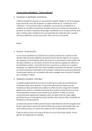
Flux flange-slab (kW/m²)
�� ��
�� ��
Figure 10_Heat fl ux from top fl ange to concrete slab during the heating phase
(left) and the cooling phase (right : t heating = 30 min) of parametrical fi re curves
The quantity of heat �Qslab exchanged between the top
fl ange and the concrete slab during a time step �t is respectively
given by Eqs 10 and 11 for 2-D beam sections (in
which bb is the width of the beam fl ange) and for 3-D joint
zones. The transfer area Atransfer is given in Eq. 12, where
tp, bp, bc and hc are the thickness of the end-plate, the
width of the end-plate, the width of the column fl ange and
the height of the column. The lengths lb and lc are taken
as equal to the half of the beam height and the half of the
column height.
� � b � �t
Qslab b
�Qslab � � Atransfer
�t
transfer
b
b
(Eq. 10)
(Eq. 11)
(Eq. 12)
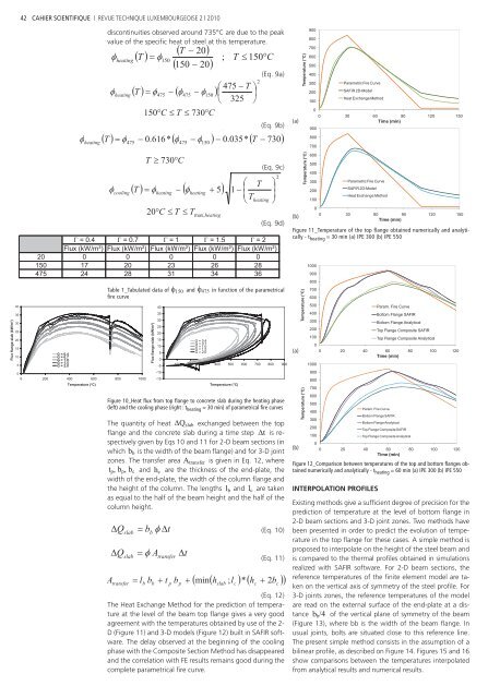
The Heat Exchange Method for the prediction of temperature
at the level of the beam top fl ange gives a very good
agreement with the temperatures obtained by use of the 2-
D (Figure 11) and 3-D models (Figure 12) built in SAFIR software.
The delay observed at the beginning of the cooling
phase with the Composite Section Method has disappeared
and the correlation with FE results remains good during the
complete parametrical fi re curve.
2
� T
1 � �
�
� T
heating
�
�
�
�
40
35
30
25
20
� �
15
10
5
0
G = 0.4
G = 0.7
G = 1.0
G = 1.5
G = 2.0
-5
0
-10
-15
100 200 300 400 500 600 700 800 900
p
p
Temperature (°C)
�min�h; l �* �h�b�� A � l b � t b �
2
slab
c
c
2
c
(a)
(b)
Time (min)
Figure 11_Temperature of the top flange obtained numerically and analytically
- theating = 30 min (a) IPE 300 (b) IPE 550
� �
(a)
Temperature (°C)
Temperature (°C)
Temperature (°C)
Temperature (°C)
900
800
700
600
500
400
300
200
100
Parametric Fire Curve
SAFIR 2D-Model
Heat Exchange Method
0
0 30 60 90 120 150
Time (min)
900
800
700
600
500
400
300
200
100
1000
Parametric Fire Curve
SAFIR 2D-Model
Heat Exchange Method
0
0 30 60 90 120 150
900
800
700
600
500
400
300
200
100
1000
� �
0
0 20 40 60
Time (min)
80 100 120
900
800
700
600
500
400
300
200
100
0
Param. Fire Curve
(b)
0 20 40 60
Time (min)
80 100 120
Figure 12_Comparison between temperatures of the top and bottom fl anges obtained
numerically and analytically - theating = 60 min (a) IPE 300 (b) IPE 550
INTERPOLATION PROFILES
Param. Fire Curve
Bottom Flange SAFIR
Bottom Flange Analytical
Top Flange Composite SAFIR
Top Flange Composite Analytical
Bottom Flange SAFIR
Bottom Flange Analytical
Top Flange Composite SAFIR
Top Flange Composite Analytical
Existing methods give a suffi cient degree of precision for the
prediction of temperature at the level of bottom fl ange in
2-D beam sections and 3-D joint zones. Two methods have
been presented in order to predict the evolution of temperature
in the top fl ange for these cases. A simple method is
proposed to interpolate on the height of the steel beam and
is compared to the thermal profi les obtained in simulations
realized with SAFIR software. For 2-D beam sections, the
reference temperatures of the fi nite element model are taken
on the vertical axis of symmetry of the steel profi le. For
3-D joints zones, the reference temperatures of the model
are read on the external surface of the end-plate at a distance
bb/4 of the vertical plane of symmetry of the beam
(Figure 13), where bb is the width of the beam fl ange. In
usual joints, bolts are situated close to this reference line.
The present simple method consists in the assumption of a
bilinear profi le, as described on Figure 14. Figures 15 and 16
show comparisons between the temperatures interpolated
from analytical results and numerical results.