TCAR - Typhoon Committee

TCAR
CHAPTER 5 - RESEARCH FELLOWSHIP TECHNICAL REPORT
as the number of samples dropped rapidly at longer
forecast range (Fig. 1).
Besides, the calibrated intensity forecasts were still not
quite able to forecast the rapid change of TC intensity
(both deepening or weakening) as evident in Fig. 4(a)
and (b).This could be attributed to model limitations in
adequately resolving the TC structure with a coarse
grid spacing of 1.125 degrees (i.e. around 120 km).
5. Probabilistic approach
A suite of methods have since been developed
for calibrating probability forecasts derived from
ensemble systems, such as multiple implementation
of single-integration MOS equations (Erickson, 1996),
ensemble dressing (Roulston and Smith, 2003) € and
logistic regression methods (Hamill et al. 2004).
Hamill and Colucci (1997, 1998) described a rank
histogram calibration based on the reliability of past
forecasts.This method has been applied to temperature
and precipitation forecasting.In this study, the same
approach was tested to post-process the probability
forecast of TC intensity category, according to the
following classification:
• Low system (LOW) – maximum wind < 22 kt
• Tropical Depression (TD) – 22 kt ≤ maximum
wind < 34 kt
• Tropical Storm (TS) – 34 kt ≤ maximum wind <
48 kt
• Severe Tropical Storm (STS) – 48 kt ≤ maximum
wind < 64 kt
• Typhoon (TY) – 64 kt ≤ maximum wind
In view of the lack of samples and relatively
unsatisfactory performance of the calibrated intensity
forecasts in the longer forecast range as discussed
in Section 4, probability forecasts as explored in this
study will be confined to the first 120 hours.
a. Methodology
The rank histogram calibration method can be divided
into two steps: bias correction and calibration.
1) Bias correction
Before constructing the rank histogram, each member
forecast was first de-biased to remove any systematic
errors in the maximum wind forecasts.Two different
methods have been tested.The first method was
simple bias removal.The correction (corr) to be made
was determined as follows:
……………….(1)
where i is the forecast range (6, 12, ......, 120-h), n
the number of samples, OBSW the BT maximum wind
speed and EMW the ensemble mean of the maximum
wind speed.
Another method
n
corr was to correct all
i = ∑(OBSWi,
j − EMWi, j )
j =1
member forecasts
using the ANN
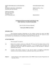
approach described in Section 4.The mean errors
of the direct EPS outputs and the corrected member
forecasts in 2005 are plotted in Fig. 5.
The mean errors after correction using both methods
described above are much reduced, falling within -5
to +5 kt for the whole forecast range.
Fig. 5 - The mean errors of the maximum wind speed
forecasts in 2005.DMO: the maximum wind speed as
derived from the direct EPS outputs; ANN: correction
by ANN described in Section 4; and SBR: correction
by simple bias removal.
2)Calibration
The bias correction described above effectively
removed the systematic biases but the corrected
probability forecasts might still not be reliable.
Following Hamill and Colucci (1997), the probability
distribution was calibrated using the verification rank
histogram.The rank histogram consisting of 24 bins
de-limited by the 25 members’ forecasts of maximum
wind were sorted in numerical order, with two
2009
273