Advanced Research WRF (ARW) Technical Note - MMM - University ...

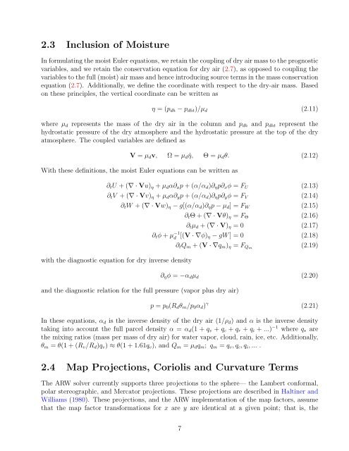
2.3 Inclusion of Moisture
In formulating the moist Euler equations, we retain the coupling of dry air mass to the prognostic
variables, and we retain the conservation equation for dry air (2.7), as opposed to coupling the
variables to the full (moist) air mass and hence introducing source terms in the mass conservation
equation (2.7). Additionally, we define the coordinate with respect to the dry-air mass. Based
on these principles, the vertical coordinate can be written as
η = (pdh − pdht)/µd
(2.11)
where µd represents the mass of the dry air in the column and pdh and pdht represent the
hydrostatic pressure of the dry atmosphere and the hydrostatic pressure at the top of the dry
atmosphere. The coupled variables are defined as
V = µdv, Ω = µd ˙η, Θ = µdθ. (2.12)
With these definitions, the moist Euler equations can be written as
∂tU + (∇ · Vu)η + µdα∂xp + (α/αd)∂ηp∂xφ = FU
∂tV + (∇ · Vv)η + µdα∂yp + (α/αd)∂ηp∂yφ = FV
∂tW + (∇ · Vw)η − g[(α/αd)∂ηp − µd] = FW
∂tΘ + (∇ · Vθ)η = FΘ
with the diagnostic equation for dry inverse density
(2.13)
(2.14)
(2.15)
(2.16)
∂tµd + (∇ · V)η = 0 (2.17)
∂tφ + µ −1
d [(V · ∇φ)η − gW ] = 0 (2.18)
∂tQm + (V · ∇qm)η = FQm
(2.19)
∂ηφ = −αdµd
and the diagnostic relation for the full pressure (vapor plus dry air)
p = p0(Rdθm/p0αd) γ
(2.20)
(2.21)
In these equations, αd is the inverse density of the dry air (1/ρd) and α is the inverse density
taking into account the full parcel density α = αd(1 + qv + qc + qr + qi + ...) −1 where q∗ are
the mixing ratios (mass per mass of dry air) for water vapor, cloud, rain, ice, etc. Additionally,
θm = θ(1 + (Rv/Rd)qv) ≈ θ(1 + 1.61qv), and Qm = µdqm; qm = qv, qc, qi, ... .
2.4 Map Projections, Coriolis and Curvature Terms
The ARW solver currently supports three projections to the sphere— the Lambert conformal,
polar stereographic, and Mercator projections. These projections are described in Haltiner and
Williams (1980). These projections, and the ARW implementation of the map factors, assume
that the map factor transformations for x are y are identical at a given point; that is, the
7