Advanced Research WRF (ARW) Technical Note - MMM - University ...

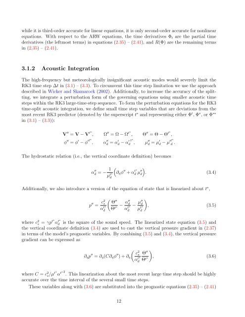
while it is third-order accurate for linear equations, it is only second-order accurate for nonlinear
equations. With respect to the ARW equations, the time derivatives Φt are the partial time
derivatives (the leftmost terms) in equations (2.35) – (2.41), and R(Φ) are the remaining terms
in (2.35) – (2.41).
3.1.2 Acoustic Integration
The high-frequency but meteorologically insignificant acoustic modes would severely limit the
RK3 time step ∆t in (3.1) – (3.3). To circumvent this time step limitation we use the approach
described in Wicker and Skamarock (2002). Additionally, to increase the accuracy of the splitting,
we integrate a perturbation form of the governing equations using smaller acoustic time
steps within the RK3 large-time-step sequence. To form the perturbation equations for the RK3
time-split acoustic integration, we define small time step variables that are deviations from the
most recent RK3 predictor (denoted by the superscript t ∗ and representing either Φ t , Φ ∗ , or Φ ∗∗
in (3.1) – (3.3)):
V ′′ = V − V t∗
, Ω ′′ = Ω − Ω t∗
, Θ ′′ = Θ − Θ t∗
,
φ ′′ = φ ′ ∗
′t
− φ , α ′′
d = α ′ d − α ′ t
d
∗
, µ ′′
d = µ ′ ∗
′t
d − µ d .
The hydrostatic relation (i.e., the vertical coordinate definition) becomes
α ′′
d = − 1
µ t∗
∂ηφ
d
′′ + α t∗
d µ ′′
d . (3.4)
Additionally, we also introduce a version of the equation of state that is linearized about t ∗ ,
p ′′ = c2s αt∗ ′′ Θ
d Θt∗ − α′′ d
αt∗ d
− µ′′ d
µ t∗
, (3.5)
d
where c2 s = γpt∗αt∗ d is the square of the sound speed. The linearized state equation (3.5) and
the vertical coordinate definition (3.4) are used to cast the vertical pressure gradient in (2.37)
in terms of the model’s prognostic variables. By combining (3.5) and (3.4), the vertical pressure
gradient can be expressed as
∂ηp ′′ = ∂η(C∂ηφ ′′ ) + ∂η
2 cs αt∗ Θ
d
′′
Θt∗
, (3.6)
where C = c2 s/µ t∗αt∗2
. This linearization about the most recent large time step should be highly
accurate over the time interval of the several small time steps.
These variables along with (3.6) are substituted into the prognostic equations (2.35) – (2.41)
12