Advanced Research WRF (ARW) Technical Note - MMM - University ...

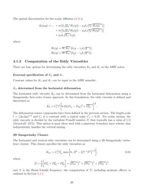
The spatial discretization for the scalar diffusion (4.5) is
where
∂t(µdq) = ... + m x
δx µd H1(q)
− µdδz zx x H1(q) xη
+ m y
δy µd H2(q)
− µdδz zy y H2(q) yη
η
+ µdδz Kv δzq ,
H1(q) = m x x
Kh δxq − zxδz(q xη ) ,
H2(q) = m y y
Kh δyq − zyδz(q yη ) .
4.1.3 Computation of the Eddy Viscosities
There are four options for determining the eddy viscosities Kh and Kv in the ARW solver.
External specification of Kh and Kv
Constant values for Kh and Kv can be input in the ARW namelist.
Kh determined from the horizontal deformation
The horizontal eddy viscosity Kh can be determined from the horizontal deformation using a
Smagorinsky first-order closure approach. In this formulation, the eddy viscosity is defined and
discretized as
Kh = C 2 s l 2
0.25(D11 − D22) 2 + D2 1
xy 2
12 .
The deformation tensor components have been defined in the previous section. The length scale
l = (∆x∆y) 1/2 and Cs is a constant with a typical value Cs = 0.25. For scalar mixing, the
eddy viscosity is divided by the turbulent Prandtl number Pr that typically has a value of 1/3
(Deardorff, 1972). This option is most often used with a planetary boundary layer scheme that
independently handles the vertical mixing.
3D Smagorinsky Closure
The horizontal and vertical eddy viscosities can be determined using a 3D Smagorinsky turbulence
closure. This closure specifies the eddy viscosities as
Kh,v = C 2 s l 2
h,v max 0., D 2 − P −1
r N 2
1/2
, (4.6)
where
D = 1
D
2
2 11 + D 2 22 + D 2
33 + xy2 xη2 yη2, D12 + D13 + D23
and N is the Brunt-Väisälä frequency; the computation of N, including moisture effects, is
outlined in Section 4.1.4.
26