Advanced Research WRF (ARW) Technical Note - MMM - University ...

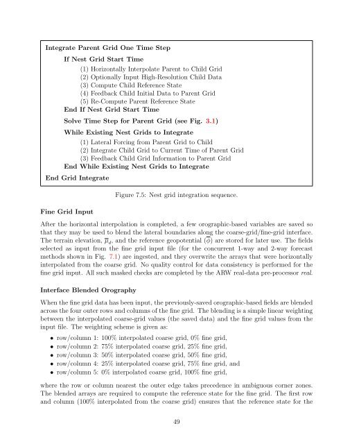
Integrate Parent Grid One Time Step
If Nest Grid Start Time
(1) Horizontally Interpolate Parent to Child Grid
(2) Optionally Input High-Resolution Child Data
(3) Compute Child Reference State
(4) Feedback Child Initial Data to Parent Grid
(5) Re-Compute Parent Reference State
End If Nest Grid Start Time
Solve Time Step for Parent Grid (see Fig. 3.1)
While Existing Nest Grids to Integrate
(1) Lateral Forcing from Parent Grid to Child
(2) Integrate Child Grid to Current Time of Parent Grid
(3) Feedback Child Grid Information to Parent Grid
End While Existing Nest Grids to Integrate
End Grid Integrate
Fine Grid Input
Figure 7.5: Nest grid integration sequence.
After the horizontal interpolation is completed, a few orographic-based variables are saved so
that they may be used to blend the lateral boundaries along the coarse-grid/fine-grid interface.
The terrain elevation, µ d, and the reference geopotential (φ) are stored for later use. The fields
selected as input from the fine grid input file (for the concurrent 1-way and 2-way forecast
methods shown in Fig. 7.1) are ingested, and they overwrite the arrays that were horizontally
interpolated from the coarse grid. No quality control for data consistency is performed for the
fine grid input. All such masked checks are completed by the ARW real-data pre-processor real.
Interface Blended Orography
When the fine grid data has been input, the previously-saved orographic-based fields are blended
across the four outer rows and columns of the fine grid. The blending is a simple linear weighting
between the interpolated coarse-grid values (the saved data) and the fine grid values from the
input file. The weighting scheme is given as:
• row/column 1: 100% interpolated coarse grid, 0% fine grid,
• row/column 2: 75% interpolated coarse grid, 25% fine grid,
• row/column 3: 50% interpolated coarse grid, 50% fine grid,
• row/column 4: 25% interpolated coarse grid, 75% fine grid, and
• row/column 5: 0% interpolated coarse grid, 100% fine grid,
where the row or column nearest the outer edge takes precedence in ambiguous corner zones.
The blended arrays are required to compute the reference state for the fine grid. The first row
and column (100% interpolated from the coarse grid) ensures that the reference state for the
49