Advanced Research WRF (ARW) Technical Note - MMM - University ...

After computing µ ′′ τ+∆τ ′′τ+∆τ
d from (3.20), Ω is recovered by using (3.9) to integrate the ∂ηΩ ′′
term vertically using the lower boundary condition Ω ′′ = 0 at the surface. Equation (3.10)
is then stepped forward to calculate Θ ′′τ+∆τ
. Equations (3.11) and (3.12) are combined to
form a vertically implicit equation that is solved for W ′′τ+∆τ
subject to the boundary condition
W ′′ = V ′′ · ∇h at the surface (z = h(x, y)) and p ′ = 0 along the model top. φ ′′τ+∆τ is then
obtained from (3.12), and p ′′τ+∆τ and α ′′
d
3.1.3 Full Time-Split Integration Sequence
τ+∆τ are recovered from (3.5) and (3.4).
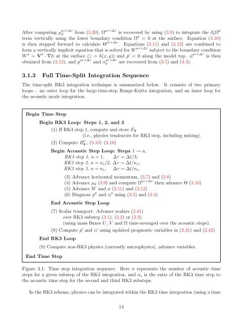
The time-split RK3 integration technique is summarized below. It consists of two primary
loops— an outer loop for the large-time-step Runge-Kutta integration, and an inner loop for
the acoustic mode integration.
Begin Time Step
Begin RK3 Loop: Steps 1, 2, and 3
(1) If RK3 step 1, compute and store FΦ
(i.e., physics tendencies for RK3 step, including mixing).
(2) Compute Rt∗ Φ , (3.13)–(3.18)
Begin Acoustic Step Loop: Steps 1 → n,
RK3 step 1, n = 1, ∆τ = ∆t/3;
RK3 step 2, n = ns/2, ∆τ = ∆t/ns;
RK3 step 3, n = ns, ∆τ = ∆t/ns.
(3) Advance horizontal momentum, (3.7) and (3.8)
(4) Advance µd (3.9) and compute Ω ′′τ+∆τ then advance Θ (3.10)
(5) Advance W and φ (3.11) and (3.12)
(6) Diagnose p ′′ and α ′′ using (3.5) and (3.4)
End Acoustic Step Loop
(7) Scalar transport: Advance scalars (2.41)
over RK3 substep (3.1), (3.2) or (3.3)
(using mass fluxes U, V and Ω time-averaged over the acoustic steps).
(8) Compute p ′ and α ′ using updated prognostic variables in (2.31) and (2.42)
End RK3 Loop
(9) Compute non-RK3 physics (currently microphysics), advance variables.
End Time Step
Figure 3.1: Time step integration sequence. Here n represents the number of acoustic time
steps for a given substep of the RK3 integration, and ns is the ratio of the RK3 time step to
the acoustic time step for the second and third RK3 substeps.
In the RK3 scheme, physics can be integrated within the RK3 time integration (using a time
14